Lecture 1: Introduction to Statistical Programming

Statistical Programming
Prof. Dr. Martin Spindler

Welcome and Motivation

Welcome to Statistical Programming with Python

About this course

Course outline
- Part I: Introduction to Programming with Python
- Part II: Data Handling, Manipulation, and Visualization
- Part III: Machine Learning - Regression
- Part IV: Machine Learning - Classification
Materials will be provided in STiNE

Welcome to Statistical Programming with Python

About this course

Teaching
- Lecture: Presentation of tools and concepts, based on examples
- Tutorial: Hands-on examples to be solved in groups; help and support
- The course is blocked ➡️ Intense phase to get started and learn basics of programming
Exam: Assignment, published on March 06, submission no later than March 20

Welcome to Statistical Programming with Python

About us

Martin Spindler:

Professor at Uni Hamburg, Chair of Statistics
Course Director
martin.spindler@uni-hamburg.de

Dr. Jan Rabenseifner:

RA at Uni Hamburg, Chair of Statistics
Lecture 2-5, Tutorials 1, 3, 4
jan.rabenseifner@uni-hamburg.de

Jan Teichert-Kluge:

RA at Uni Hamburg, Chair of Statistics
Lecture 1
jan.teichertkluge@uni-hamburg.de

Valerian Fourel:

RA at Uni Hamburg, Chair of Statistics and HCHE
Tutorial 2
valerian.fourel@uni-hamburg.de

We really appreciate active participation and interaction!

Welcome to Statistical Programming with Python

The assignment

You will be given several statistical programming exercises you have to solve with Python
You can group up (4 students) and work together. Each student group submits one solution. Please, provide your name on your solution
Your solution:
- A report or presentation (.pdf) summarizing your solution to the statistical problem
- You provide a code solution to the problem
- Code files need to be executable
I’d encourage you to start and submit your solution early and to use Quarto

Welcome to Statistical Programming with Python

What to expect

We’ll cover the basics of programming (in Python) at the beginning
- This is really similar to learning a new foreign language
- First, you have to get used to the language and learn basic words
- Later, you’ll be able to apply the language and see some results
- Similar to learning a language: Practice, practice, practice!
- So: Expect some investment in the beginning and to see the return later

Welcome to Statistical Programming with Python

What to expect

After completing the course, you will be able to read code and write your own program using Python
- That’s quite something
- You can ask questions and get support during the lecture and tutorials
In addition to a standard programming course, you’ll learn how to use Python for statistical problems
You can see this as a rough introduction to the basics of data science

What is Statistical Programming?

The term statistical programming refers to the process of writing code in a programming language in order to perform a statistical analysis. There are various softwares available that are different, e.g., in terms of programming effort, efficiency and implemented methods. The most widely used softwares to perform statistical analysis by machine learning methods are R and Python.

Statistical programming combines two elements:

Knowledge of statistical methods
Knowledge of programming techniques

What is Statistical Programming?

Exemplary tasks

Summarize and display data, e.g., generate plots like histograms or scatter plots, calculate descriptive statistics, exploratory data analysis
Fit a statistical model to data, e.g., to predict an outcome of interest
Simulations, e.g., to verify statistical properties of estimators

Motivation: Why learn programming?

Statistical Analysis
Machine Learning
Data Visualization
Problem Solution

About this course

Goals

Essential concepts and tools of modern programming
Automated solutions for recurrent tasks
Algorithm-based solutions of complex problems
Application of programming in statistical / data science problems
“Use AI” in a specific context

Language

Python (3), but the concepts expand to other languages, too!
A good language to get started
Can be used for a wide variety of tasks
Heavily used in industry and research (data science, AI)

How to learn programming

My recommendation for this course

Hear: Attend lecture
See: Read lecture notes and examples yourself, read up in corresponding book chapters to fully understand
Do: Run code examples on your own, play around, google/find help, modify, solve problem sets

The learning path can be quite hilly

Programming is problem solving, but don’t get frustrated too easily!
Learn something new and useful: Expect to stretch your comfort zone
Some statistical concepts can be quite complex: Use programming to pragmatically approach them

How to learn programming

The learning path can be quite hilly

Collaborate with your colleagues and figure out solutions together: Help each other :-)
Try to find help: Lecture materials and books, Python (library) documentation, online (google, ChatGPT, StackOverflow.com)

source: c-sharpcorner.com

How to learn programming

The learning path can be quite hilly

In case you get frustrated, read this nice little blog post about this (medium.com).

Literature

Books

Wentworth et al. (2015): How to Think Like a Computer Scientist: Learning with Python 3, Release 3rd Edition, 2017, available online
Porter and Zingaro (2024): Learn AI-Assisted Python Programming with GitHub Copilot and ChatGPT.
Downey (2012): Think Python, 2nd Edition, available online

Errata

In case you find errors and typos in the lecture notes, please report them in the form on the course website.

Getting started

Let’s get started!

Setting up Python on your machine

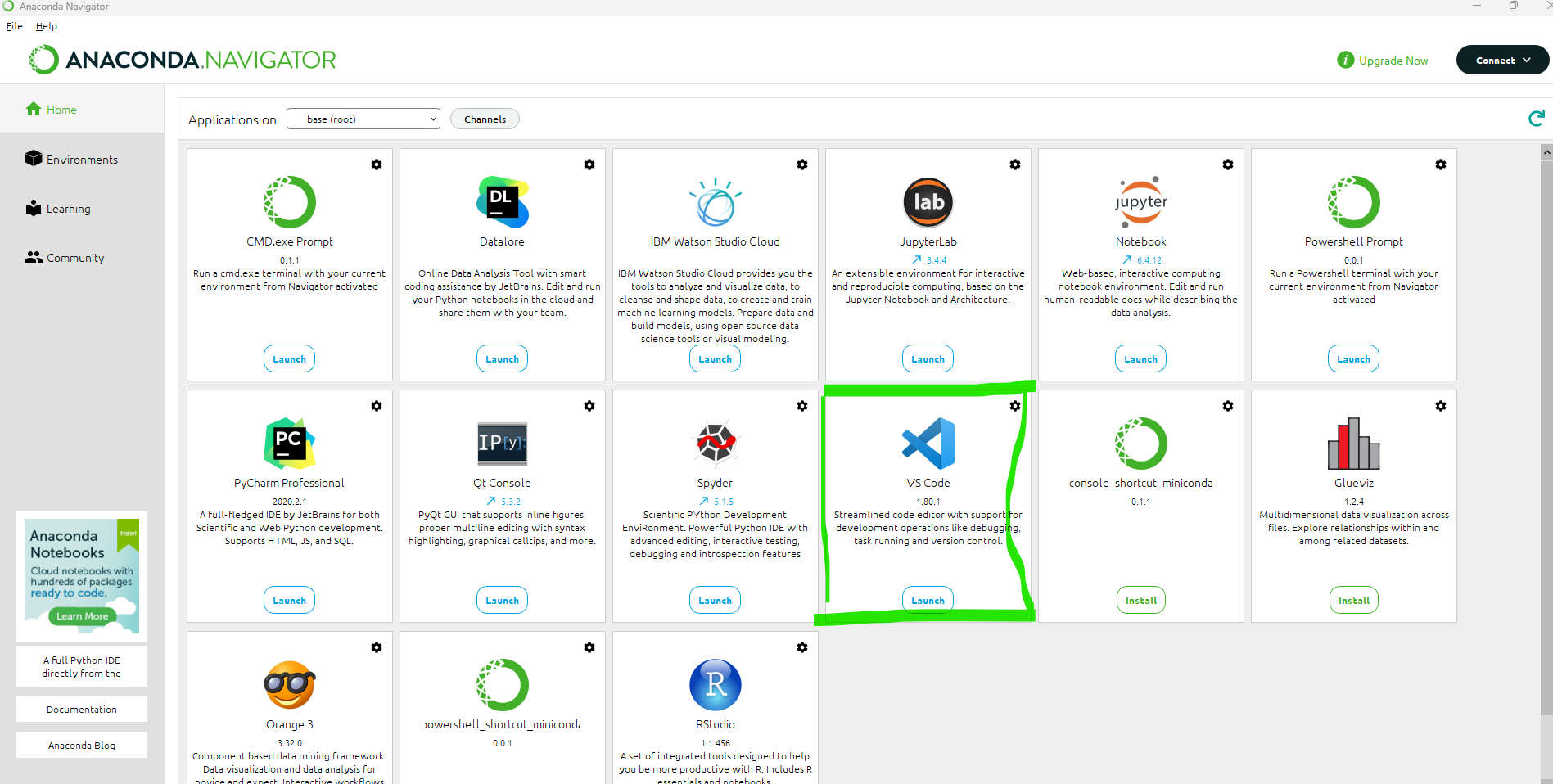
Option 1: Anaconda (Traditional)

Install latest version of Anaconda on your laptop
- Installation guide for Windows
- Installation guide for MacOS
Comes with many pre-installed packages
Good for beginners

Option 2: UV (Modern & Fast)

Install UV: docs.astral.sh/uv
10-100x faster than pip/conda
Modern Python package and project manager
Recommended for new projects

Setting up your Editor

Editor: VS Code

Download VS Code
Install Python extension
Works with both Anaconda and UV

Editor: Positron

Download Positron
Positron is a next-generation, open-source IDE developed by Posit, specifically designed for data science
Since it is a fork of Code OSS, you can use most VS Code extensions and themes, providing a familiar and highly customizable environment.

Modern Python Tooling: UV

Why UV?

Fast: 10-100x faster than pip/conda
Modern: Single tool for everything
Simple: No separate venv management
Reliable: Deterministic dependency resolution

Installation

# Windows (PowerShell)
powershell -ExecutionPolicy ByPass -c "irm https://astral.sh/uv/install.ps1 | iex"

# macOS/Linux
curl -LsSf https://astral.sh/uv/install.sh | sh

Quick Start with UV

# Create a new project
uv init my_project
cd my_project

# Add dependencies
uv add numpy pandas matplotlib scipy scikit-learn

# Run Python
uv run python script.py

# Start interactive Python
uv run python

Learn More

UV vs Traditional Tools

Traditional Workflow (pip/conda)

# Create virtual environment
python -m venv myenv
source myenv/bin/activate  # or myenv\Scripts\activate on Windows

# Install packages
pip install numpy pandas matplotlib
# Wait... wait... wait...

# Manage dependencies
pip freeze > requirements.txt

# Reproduce environment
pip install -r requirements.txt

Modern Workflow (UV)

# Everything in one command
uv add numpy pandas matplotlib
# Done in seconds!

# Dependencies auto-managed
# pyproject.toml + uv.lock created

# Reproduce environment
uv sync
# Fast and deterministic

Key Advantages

No separate venv commands needed
10-100x faster package installation
Automatic dependency locking
Single tool for everything

Modern Python Project Structure

Project created with UV

my_project/
├── pyproject.toml      # Project metadata & dependencies
├── uv.lock            # Locked versions (like package-lock.json)
├── .python-version    # Python version for project
├── src/
│   └── my_project/
│       └── __init__.py
└── README.md

pyproject.toml (Modern standard)

[project]
name = "my_project"
version = "0.1.0"
dependencies = [
    "numpy>=1.26.0",
    "pandas>=2.1.0",
    "matplotlib>=3.8.0"
]

[tool.uv]
dev-dependencies = [
    "pytest>=7.4.0",
    "ruff>=0.1.0"
]

Key Benefits

pyproject.toml: Single source of truth
- Replaces setup.py, requirements.txt, etc.
- Industry standard (PEP 621)
uv.lock: Reproducible builds
- Exact versions locked
- Fast dependency resolution
Easy commands

# Install all dependencies
uv sync
# Add new package
uv add scikit-learn
# Update packages
uv lock --upgrade
# Run scripts
uv run python analysis.py
# Run tests
uv run pytest

AI-Assisted Coding

Why Use AI Coding Assistants?

Faster Development: Auto-complete code blocks
Learning Tool: Understand new libraries/patterns
Debug Helper: Find and fix errors quickly
Documentation: Generate docstrings and comments
Best Practices: Learn idiomatic code patterns

Example Use Cases

# Type a comment, AI suggests implementation
# Function to calculate mean and std of a list

# AI suggests:
def calculate_stats(data):
    mean = sum(data) / len(data)
    variance = sum((x - mean)**2 for x in data) / len(data)
    std = variance ** 0.5
    return mean, std

Popular Tools

GitHub Copilot: IDE integration, code suggestions
Claude Code (CLI or Desktop): Orchestrated, autonomous tasks
ChatGPT/Claude: Code generation, debugging help
Cursor: AI-first code editor

GitHub Copilot & Claude Code

GitHub Copilot

Integrated into VS Code, JetBrains IDEs
Real-time code suggestions as you type
Multi-line completions
Test generation
Free for students/educators

Tips

Write descriptive comments first
Use clear function/variable names
Accept suggestions with Tab
Cycle through alternatives

Claude Code (CLI Tool)

Autonomous coding in terminal
Can read/edit multiple files
Executes commands, runs tests
Great for refactoring/bug fixes

Setup & Usage

# Install Claude Code CLI
npm install -g @anthropic-ai/claude-code
# Basic usage
claude "add type hints to all functions"
# Interactive mode
claude

When to Use

Bulk refactoring tasks
Writing boilerplate code
Setting up project structure
Code reviews and optimization

Responsible AI Usage in Coding

✅ Good Practices

Learn from AI suggestions
- Understand why code works
- Study patterns and idioms
- Ask AI to explain complex parts
Verify outputs
- Test all AI-generated code
- Check for edge cases
Incremental adoption
- Start with simple tasks, increase complexity
- Build your own expertise
Cite when needed
- Acknowledge AI assistance in projects
- Follow academic integrity guidelines

❌ Avoid These Pitfalls

Blind copy-paste
- Don’t use code you don’t understand
- Can introduce bugs or vulnerabilities
Over-reliance
- Build your own problem-solving skills
- Practice coding without AI regularly
Sensitive data
- Don’t share proprietary code
- Avoid sending personal/confidential data
- Check your organization’s AI policy
Academic dishonesty
- Follow your institution’s rules
- Understand assignment requirements
- AI is a tool, not a substitute for learning

AI Coding: Practical Examples

Example 1: Data Analysis Task

# Prompt to AI: "Load CSV file and compute
# descriptive statistics for all numeric columns"

# AI generates:
import pandas as pd

def analyze_csv(filepath):
    """Load CSV and compute statistics."""
    df = pd.read_csv(filepath)
    numeric_cols = df.select_dtypes(
        include=['number']).columns

    stats = df[numeric_cols].describe()
    return stats

# You learn: pandas data type selection,
# describe() method, clean function structure

Example 2: Debugging Help

# Your buggy code:
def calculate_mean(numbers):
    return sum(numbers) / len(numbers)

# Fails with empty list!

# Ask AI: "Fix this function to handle edge cases"

# AI suggests:
def calculate_mean(numbers):
    """Calculate mean, handling edge cases."""
    if not numbers:
        return 0  # or raise ValueError
    return sum(numbers) / len(numbers)

# You learn: Input validation,
# error handling patterns

Example 3: Writing Tests

Ask AI: “Write pytest tests for calculate_mean”

AI generates tests for normal cases, edge cases, and error handling.

Learning Workflow with AI

Effective Learning Strategy

Try it yourself first
- Attempt to solve the problem
- Build problem-solving skills
- Identify what you don’t know
Use AI as a tutor
- Ask for explanations, not just code
- Request step-by-step breakdowns
- Learn the “why” behind solutions
Experiment and modify
- Change AI-suggested code
- Test different approaches
- Make it your own

Practice without AI
- Regular coding exercises
- Timed challenges
- Build muscle memory

Prompt Engineering for Coding

Good prompts get better results:

❌ Bad: "write code for data analysis"

✅ Good: "Write a Python function that:
1. Loads a CSV file using pandas
2. Handles missing values by dropping rows
3. Calculates mean and median for numeric columns
4. Returns results as a dictionary
5. Includes type hints and docstring"

Iterative refinement

1. "Write a function to sort a list"
2. "Add error handling for non-list inputs"
3. "Support custom comparison key"
4. "Add unit tests with pytest"
5. "Optimize for large lists"

AI Tools Comparison

Tool	Best For	Free?	Integration
GitHub Copilot	Real-time suggestions	Students/Edu	VS Code, JetBrains
Claude Code	Autonomous tasks	Free tier	CLI, VS Code
ChatGPT	Learning & explanations	Free tier	Web, API, Codex in VS Code
Cursor	AI-first editing	Free tier	Standalone IDE

Start with ChatGPT/Claude for learning concepts
Add GitHub Copilot or Claude Code for coding
Try Claude Code for project setup and refactoring

Part I: Introduction to Programming with Python

Let’s get started!

Running Python on your machine

VS Code is an Source Code Editor
- Short tutorial on VS Code
- Install the Python extension in VS Code (click on the extension icon on the left side) to extend VS Code to have IDE (= Integrated Development Environment) like features

Let’s get started!

Why using an IDE?

You can run Python basically using the command line
- Open a new Terminal, type python and then run following code

Code

print('hello world!')

hello world!

However, in case you want to write more complex code, it’s worth to organize your code in scripts (.py files)
IDE’s provide extra functionalities that help you write and organize your code (and software project)
- Other examples of IDE’s: PyCharm, RStudio, Spyder

Digression: Jupyter Notebooks

Notebooks are also very popular, for example Jupyter Notebooks as they …

… are very easy to share / integrate,
… are easy to replicate,
… show the code and the ouput,
… share some nice features, like markdown syntax and maths formula.

Digression: Quarto

Quarto is a new publication tool that combines the advantages of notebooks and IDE’s
You can use it now only to generate (Jupyter) Notebooks, but also to generate books, websites and slideshows
The more familiar you are with Python, you will find it more easily to also use other tools like Jupyter and Quarto
We will focus on using VS Code in this course. If you are interested, we can demonstrate Jupyter and Quarto later in the course
We recommend you to use Quarto for your assignment solution

Let’s get started!

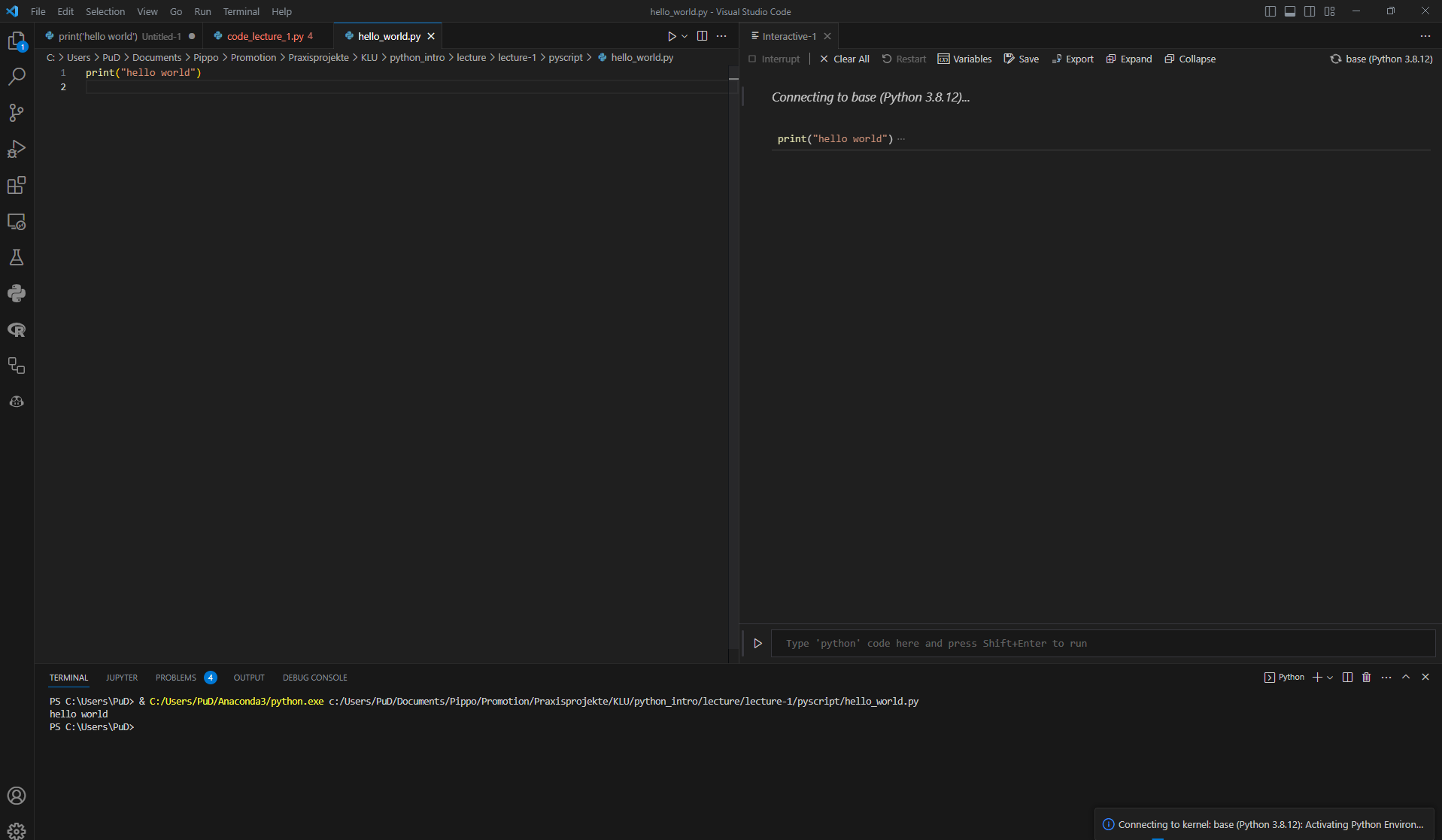
It’s time for our first code example

From VS Code

Open VS Code
Create a new file called hello_world.py (click on file > new file)
Save the file
- Recommended: Open / create a new directory where you save your .py files

Insert the following code in the file

Code

print("hello world")

x = [1,4,5]

hello world

Execute this code on your laptop (go to line and press Shift + Enter) or click on the Run button on the top right

Let’s get started!

It’s time for our first code example

In Terminal / Interactive Window

Copy the code from hello_world.py
Go to the Terimnal, type python and paste the code
Execute the code by pressing Enter

Alternatively you can click on the Interactive Window button on the top right and paste the code there

Let’s get started!

It’s time for our first code example

Using the command line (without IDE)

Open the command line
- Windows: Press windows key and enter cmd or open Anaconda Prompt
- Mac: Open terminal
Direct to the directory with hello_world.py using cd
Type python hello_world.py

Let’s get started!

Congratulations!

You just ran your first Python code example!

via GIPHY

Introduction to Programming with Python

What is a program?

A program is a sequence of instructions that specifies how to perform a computation (mathematical or symbolic)
Basic instructions in virtually any language
- Input: Get data from keyboard, file, network, …
- Output: Display data on screen, save in file, send to network, …
- Math: Perform basic mathematical operations, …
- Conditional execution: Check for certain conditions and run appropriate code
- Repetition: Perform some action repeatedly (with some variation)

Programming: Process of breaking a large, complex task into smaller and smaller substasks until the subtask is simple enough to be performed with one of these basic instructions (Downey, 2015, P. 2)

Print command

Typical first example

Code

# Print 'hello world!'
print("hello world!")

hello world!

print() function: Displays a value on the screen
Quotation marks don’t show up in output
Comments: Can be inserted after a #, are ignored by the interpreter, only intended for human readers

Values and data types

Value: One of the fundamental things (like letter or number) that a program manipulates
Values are categorized in different classes
- integer (e.g., 4)
- string (e.g., "hello world!" or 'banana')
- float (floating point, e.g., 3.2)

Code

print(type("hello world!"))
print(type(123))
print(type("123"))
print(type(3.14))

<class 'str'>
<class 'int'>
<class 'str'>
<class 'float'>

Variables

Variables: A name that refers to a value
Assignment using the = token ( does not mean equal !)

Code

message = "What's up, Doc?"
n = 17
pi = 3.14159

Code

n**2

Variables

Some rules for variable assignment
- Case-sensitive
- Can contain letters and numbers
- Must start with a letter
- Some Python-specific keywords are reserved: def, and, class, …
- Recommended to use names that are meaningful to humans

Code

Day = "Tuesday"
print(day)

---------------------------------------------------------------------------
NameError                                 Traceback (most recent call last)
Cell In[7], line 2
      1 Day = "Tuesday"
----> 2 print(day)

NameError: name 'day' is not defined

Statements and expressions

Statement: Instruction that the Python interpreter can execute, for example, assignments, while, if, for, import
Expressions: Combination of values, variables, operators and calls to functions
- If you type an expression at the Python prompt, the interpreter evaluates it and displays the results
- The evaluation of an expression produces a value (expressions can appear on the right hand side of an assignment statement)

Code

# An expression
len('hello')

# An expression on the RHS of an assignment
x = len('hello')
print(x)

Arithmetic operators

Addition: +
Substraction: -
Multiplication: *
Division: /
Exponentiation: **
Module: %
Floor Division: //

Code

print(3**2)
print(2 + 4 - 2*10)

9
-14

Operations for strings

Strings comprise characters, i.e., single symbols of a chosen font
Strings are immutable
We can manipulate single characters in a string

Code

my_string = "Intro to Python"
print(my_string[2])

Get length of a string

Code

len(my_string)

Slicing a string with [n:m], n is included and m is excluded
- Special cases: [:m], [n:], [:]
- What happens for [-2:-1]?
- Indexing in Python starts with [0]!

Operations for strings

Slicing

Code

print(my_string[0:3])
print(my_string[3:])
print(my_string[:-1])

Int
ro to Python
Intro to Pytho

Strings are immutable!

Code

my_string[0] = "A"

---------------------------------------------------------------------------
TypeError                                 Traceback (most recent call last)
Cell In[13], line 1
----> 1 my_string[0] = "A"

TypeError: 'str' object does not support item assignment

More operations
- Testing with in and not in
- Index of a character with .find()
- Split into a list of strings using .split()

Operations for strings

Comparison of strings with: ==, > and <

Code

a = ""

Test for characters with in and not

Code

word1 = "banana"
print("a" in word1)
print("y" not in word1)

True
True

Get an index of a character with find

Code

word1.find("a")

Operations for strings

Traverse a string

Code

for letter in my_string:
    print("Give me a", letter)

Give me a I
Give me a n
Give me a t
Give me a r
Give me a o
Give me a  
Give me a t
Give me a o
Give me a  
Give me a P
Give me a y
Give me a t
Give me a h
Give me a o
Give me a n

Operations for strings

f-strings: Combine text and variables

Code

first_name = "Peter"
last_name = "Wright"
full_name = f"{first_name} {last_name}"
print(full_name)

Peter Wright

Concatenation: +

Code

print(first_name + last_name)

PeterWright

Repetition: *

Code

first_name*3

'PeterPeterPeter'

Formatting strings

Use of placeholders

Code

"I am {0} and I am an {1}".format("Philipp", "Economist")

'I am Philipp and I am an Economist'

Add format specifications,
- Alignment left (<), center (^), right(>)
- Allocated width by a number
- Type conversion to float
- Number of decimals

Code

txt = "You are {:<8} years old."
print(txt.format(123))

txt = "Pi {:.2f}."
print(txt.format(3.141529))

You are 123      years old.
Pi 3.14.

Tuples

Tuples are collections of values

Code

record = ("Bolt", 9.58, 100, "Jamaica")

Assignment analogously to strings

Code

(name, time, distance, country) = record

Nested tuples are possible
Tuples are immutable (like strings)

Lists

Lists are generalizations of strings, i.e., an ordered collection of values
- not restricted to characters and not restricted to a single type

Code

height = [8.848, 8.611, 8.586]
names = ["Mount Everest", "K2", "Kangchenjunga"]
everest = [8.848, "Mount Everest"]

Lists

Operations on lists
- in and not in
- Accessing as for strings
- Concatenation + and repetition *
- len() for length
- Lists are mutable

Code

numbers = [1, 2, 3, 4]
numbers[0] = 42
print(numbers)

[42, 2, 3, 4]

Lists

Empty lists with []
Nested lists, e.g., [1, 2, [4, 5]]
Remove elements from lists using del

Methods for lists

Method: A function attached to an object. Invoking (= activating) a method causes the object to respond in some way, in Python using . notation.
Object here: list
Methods:
- .append(element): Add element to end of the list
- .insert(position, element): Adds element at position and shifts remaining elements up
- .count(element): Counts how often element appears in a list
- .extend(newlist): Puts newlist at the end of the list

Methods for lists

Method: A function attached to an oject. Invoking (= activating) a method causes the object to respond in some way, in Python using . notation.
Object here: list
Methods:
- .index(element): Finds the index of the first time element apears in the list
- .reverse()
- .sort()
- .remove(element): Removes element at the first position it appears

Lists are mutable objects

Example

Code

names2 = names
names2[0] = "Mount Denmark"

print(names)

['Mount Denmark', 'K2', 'Kangchenjunga']

What happened here?
- Aliasing \(\neq\) Cloning
- Aliasing: Assign two lists to the same object / memory
- Cloning: Generate a copy of an existing list, .copy() or use slicing [:]

Lists are mutable objects

Test whether two names refer to the same object using is

Code

names3 = names2.copy()
names3[0] = "Machu Picchu"

print(names3 is names2)
print(names2 is names)
print(names3)
print(names2)

False
True
['Machu Picchu', 'K2', 'Kangchenjunga']
['Mount Denmark', 'K2', 'Kangchenjunga']

Dictionaries

Dictionaries are mappings from keys of immutable type to values of any (heterogeneous) type
Use key:value pairs to define dictionaries and add pairs with [] or .update({key:value}).

Code

mycar = {
  "brand": "Ford",
  "model": "Mustang",
  "year": 1964
}

mycar["hp"] = 210

print(mycar)

{'brand': 'Ford', 'model': 'Mustang', 'year': 1964, 'hp': 210}

Access to dictionaries is very fast
Order of pairs does not matter
- Try out .sort()!

Dictionaries

More on dictionaries
- .keys(): creates list of underlying keys
- .values(): creates list of underlying values
- .items(): creates list of key:value pairs
- in and not in test only for keys (!)
- .copy(): Create a copy of a dictionary
- .update(): Creates new entries in the dictionary or update existing ones. Allows multiple creations or updates.

Composition

So far, elements of a program have been considered in isolation

One of the most useful features of programming languages is their ability to take small building blocks and compose them into larger chunks (Wentworth et al., 2017, P. 19)

Errors and debugging

Bugs: Programming errors
Debugging: Process of tracking down errors

Programming, and especially debugging, sometimes brings out strong emotions. If you are struggling with a difficult bug, you might feel angry, despondent, or embarrassed.

[…]

Preparing for these reactions might help you deal with them. One approach is to think of the computer as an employee with certain strengths, like speed and precision, and particular weaknesses, like lack of empathy and inability to grasp the big picture (Downey, 2015, P. 6)

Errors and debugging

Bugs: Programming errors
Debugging: Process of tracking down errors

via GIPHY

Errors and debugging

Syntax error
- Violation of rules on the structure of the program
- Returning an error message and quitting the interpretation
Runtime error
- Exception occurs after the program has started running (i.e., after successful interpretation)
Semantic error (meaning)
- The program runs successfully but does not produce the desired output
- No error message
- Indications only based on output

Errors and debugging

Debugging
- Change a buggy program to a running program
- Make a running program do what you want
- Trial and error

Functions

Function: Named sequence of statements that performs a computation
Structure of functions in Python:
- def <functionname>:
- new line starts with indented body
Call function by name

Code

# Built-in function in Python
type(42)

# Define your own function
def print_lyrics():
    print("I'm a lumberjack, and I'm okay.")

print_lyrics()

I'm a lumberjack, and I'm okay.

Functions

Arguments: Functions might require arguments
Parameters: Inside a function, the arguments are assigned to (local) variables which are called parameters

Code

# Example with one argument
def print_times_two(x):
    print(x*2)

print_times_two(10)

Variables and parameters are local

Variables that are created inside a function are local, i.e., they only exist inside the function

Code

# Example with one argument and one parameter
def print_times_two(x):
    y = x*2
    print(y)

print_times_two(10)

You can try to print the variable y. Good luck!

Defaults

You can set default values for function arguments

Code

def print_times_two(x = 1):
    y = x*2
    print(y)

print_times_two()

Functions

Return values

Distinguish: Fruitful and void functions
- Void functions: Do something useful without returning a value. Python returns the value None
- Fruitful functions: Return data type that is determined by the function, specified via return statement

Code

def square1(number):
    result = number**2
    return result

squared_number = square1(10)
squared_number

Remember: Local variables exist only inside functions. Parameters are local variables.
Local variables exist only while the function is being executed. We can override this with global.

Functions and lists

Modifiers

Lists are passed as objects \(\Rightarrow\) Possible (un)intended side effects (mutability)

Code

def list_reverse(alist):
    alist.reverse()
    return alist

my_list = [0, 1, 2, 3]

my_list2 = list_reverse(my_list)
print(my_list)
print(my_list2)

[3, 2, 1, 0]
[3, 2, 1, 0]

Development

Code

def square(number):
    """
    Compute the square of a number
    """
    return 0.0

Start with skeleton and complete function step by step
Use temporary variables for checks
Once the function is completed, try to improve the code
Use print() for debugging
- Work with examples, where the solution is known in advance.
- Avoid using input or print in function bodies unless necessary (or for debugging)

Lambda Functions

A lambda function is a short anonymous function with only one expression
Use lambda as keyword to create a lambda functions.

Code

# As function:
def relu(x):
    x_r = max(x, 0)
    return x_r

print(relu(2))
print(relu(-3))

# Same as lambda function:
relu_lambda = lambda x: max(x, 0)

print(relu_lambda(2))
print(relu_lambda(-3))

Lambda functions are useful for using in higher-order functions, e.g. in .apply() for data frames.

Style

Limit line length
Name variables and functions with lowercase_letters_with_underscores (CamelCase is for classes)
Place import and function definitions at the top of a file
Place top level statements at the bottom of the file
Use docstrings for documentation
Use blank lines for separation

Why use functions?

Make code easier to read and debug
Make program smaller by avoiding code replications
Well-written functions can be reused

Modules

Modules contain a collection of functions
Modules play an important role for Python
More on this later

Functions

Docstrings

docstrings are the key way to document functions in Python

Code

def print_times_two(x = 1):
    """
    Multiplication by two
    input: x
    output: Product of x with 2
    """
    y = x*2
    print(y)

Docstring should contain information about
- Arguments
- What does it do?
- Expected result

Conditions and recursion

Execute code depending on a condition: if
Boolean expressions: An expression that is either true or false
- Equal: ==
- Not equal: !=
- Greater/less than: >, <
- Greater than or equal / less than or equal: >=, <=

Code

x = "abc"
print(len(x) == 3)
print(len(x) == 4)

True
False

Logical operators

Meaning of these operators is similar to their meaning in English: and, or, not

Code

2 < 4

True

Code

4 < 2

False

Code

4 > 2 and 4 > 1

True

Code

4 > 2 and 4 < 1

False

Conditional execution

Conditional execution based on an if statement

Source: Wikipedia

Conditional execution

Conditional execution based on an if statement
Condition: Boolean expression after if

Code

if x > 0: # Boolean expression
    print("x is positive") # Statement (after indent)

Alternative execution

Code

if x > 0:
    print("x is positive")
else:
    print("x is odd")

Placeholder statement: pass (block of statements must never be empty!)
Statement to exit the loop: break

Conditional execution

Chained conditionals

Code

if x < y:
    print("x is less than y")
elif x > y:
    print("x is greater than y")
else:
    print("x and y are equal")

Nested conditionals

Code

if x == y:
    print("x and y are equal")
else:
    if x < y:
        print('x is less than y')
    else:
        print('x is greater than y')

Recursion

Functions might call themselves

Code

def countdown(n):
    if n <= 0:
        print("Blastoff")
    else:
        print(n)
        countdown(n-1)

Code

countdown(0)

Blastoff

Caution: Infinite recursion!

Iteration

Iteration: Run a block of statements repeatedly based on for and while
Reassignment: Reassign the value of some variable (use with caution!), e.g.,

Code

a = 8
a = 4
print(a)

Updating variables: New value of a variable depends on old value

Code

# increment
a = a + 1
print(a)

# decrement
a = a - 1
print(a)

5
4

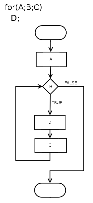
for loops

for loop: looping statements through an explicit counter / loop variable, which is specified via range()

Code

for i in range(1,10,2): # define sequence of values
    print(i) # statement

for loops

while statement:
1. Determine if condition is true or false
2. If false: continue at the next statement
3. If true: run body and go back to step 1.

Code

x = 3
while x > 0: # Boolean statement
    print(x**2) # Statement
    x = x - 1
else:
    print("x=0")

9
4
1
x=0

for loops

Using the += and -= operators in Python

Code

for u in range(2):
    u -= 1
    for i in range(2):
        i += 1
        print("i = ", i, "u = ", u)

i =  1 u =  -1
i =  2 u =  -1
i =  1 u =  0
i =  2 u =  0

Loops over lists

Code

ingredient_list = ['oregano', 'tomatoes', 'mozzarella']

for ingredient in ingredient_list:
    print("Do we have", ingredient, "?")

Do we have oregano ?
Do we have tomatoes ?
Do we have mozzarella ?

Alternatively, use the range() function

Code

for i in range(0, len(ingredient_list)):
    print("Do we have", ingredient_list[i], "?")

Do we have oregano ?
Do we have tomatoes ?
Do we have mozzarella ?

Loops over lists

Loop in reversed order

Code

for ingredient in reversed(ingredient_list):
    print("Do we have", ingredient, "?")

Do we have mozzarella ?
Do we have tomatoes ?
Do we have oregano ?

Alternatively, use the range() function

Code

for i in range(len(ingredient_list)-1, -1, -1):
    print("Do we have", ingredient_list[i], "?")

Do we have mozzarella ?
Do we have tomatoes ?
Do we have oregano ?

Files, Modules and Classes

Files

All previous programs stored data in RAM
In order to make data accessible independently from the code, we need to write it to a storage medium
Locations of certain sets of data is stored in so-called files
We have to open and close files actively for writing or reading

Files

Code

with open("test_output.txt", "w") as output:
    output.write("My first file\n")
    output.write("-------------\n")
    output.write("Hello World! \n")

with statement: secures closing of the file
open function with parameters filename and mode
w means opening for writing
output is the file handle (not the same as the file)
We call methods/functions to modify the file via the handle, but changes happen on the file
test_output.txt is created or, if it already exists, replaced with a new one (Caution!)

Files

“A handle is somewhat like a TV remote control” (Wentworth et al. (2015), P. 140)

Perform operations (switch, mute, …) on the remote (= the handle), but the real action happens on the TV

Files

Access the file using option r (reading mode)

Code

with open("test_output.txt", "r") as my_handle:
    file_lines = my_handle.readlines()

Code

with open("test_output.txt", "r") as my_handle:
    content = my_handle.read()

Directories

File system is organized in terms of directories, which contain files and further directories
So far, we have been using the current directory of the respective Python-file
To access files in different directories, we have to specify the full path:
- Windows: c:/temp/file.txt
- Linux/MacOS: :/home/Python/file.txt
- Reading/writing to files from URL works analogously

Modules

Recall: Methods for strings and lists
Modules contain definitions and statements for specific parts of programs
Anaconda comes with a lot of extra modules

Example

Random numbers

Code

import random

rng = random.Random()
coin_toss = rng.randrange(2)
print(coin_toss)

import includes all definitions and statements from the module called random
rng is the random number generator.
randrange() returns a random integer.
rng is only pseudo-random, i.e., generation based on a deterministic algorithm
seed value: Starting point, ensures repeatability for testing purposes

Code

import random

rng2 = random.Random(123)
coin_toss2 = rng2.randrange(2)
print(coin_toss2)

Math

The math module is a collection of common mathematical functions

Code

import math
print(math.pi)
print(math.sqrt(2.0))

3.141592653589793
1.4142135623730951

Variations

Standard way (load entire module)

Code

import math

Specific parts

Code

from math import sqrt
x = sqrt(25)

All into current namespace¹

Code

from math import *
x = sqrt(25)

Variations

Changing the name

Code

import math as m
x = m.sqrt(25)

We will find out how to create our own module later!
Popular examples for modules (more on this in part 2 of this course)
- numpy
- pandas
- matplotlib
- scikit-learn

Installation of modules

With UV (Recommended)

# Add a package to your project
uv add <module_name>

# Add multiple packages
uv add numpy pandas matplotlib

# Add for development only
uv add --dev pytest ruff

Faster dependency resolution
Automatic virtual environment
Lock files for reproducibility

With Anaconda/pip (Traditional)

# Using conda
conda install <module_name>

# Using pip
pip install <module_name>

# Multiple packages
pip install numpy pandas matplotlib

Anaconda comes with many pre-installed modules
See Anaconda package list

Classes and Objects

So far, we have seen the built-in data types available in Python
- character, float, string, list, …
However, we can also define our own data type, just as we can define our own functions
So far: We used functions in order to process data (= procedural programming)
Object-oriented programming(OOP): Objects contain data and functionality
OOP makes maintenance and modifitcation of (large) projects much easier

Classes and Objects

What is a class?

Class: User-defined compound data types
Define a class

Code

class Student:
    def __init__(self):
        self.mat_num = 0
        self.name = ''
        self.program = ''

Convention: Class definitions are at the beginning of a file (or in a separate module) and the name of the class starts with a capital letter (CamelCase)
- Be careful with identation levels
- __init__ : Initializer method, which is called every time a new instance of the class is created.
- self: Refers to the newly created object

Classes and Objects

Code

programmer1 = Student()
programmer2 = Student()

print('Matriculation number \n -------------\n{0:9}\n{1:9}'.format(programmer1.mat_num, programmer2.mat_num))

Matriculation number 
 -------------
        0
        0

Student() is called a constructor
Constructor and initialization method lead to an instance: “Create a new object and set it to default values”

Classes and Objects

Modify and Improve

Accesss and modify an attribute using Python’s dot notation

Code

programmer1.mat_num = 12345678
programmer2.program = 'k-nearest neighbor'

print(programmer1.mat_num)
print(programmer2.program)

12345678
k-nearest neighbor

Improve initialization (reduce number of lines for instantiation, add documentation)

Code

class Student:
    """Student class with essential data"""
    def __init__(self, num=0, name='', program=''):
        """Create a new student object"""
        self.mat_num = num
        self.name = name
        self.program = program

programmer3 = Student(87654321, '', 'lasso shooting fit')

Classes and Objects

Methods

Methods: Operations to the class, which are specific to our data structure

Code

class Point:
    """Creates point with coordinates x,y"""
    def __init__ (self, x=0, y=0):
        """Create a new point at (x,y)"""
        self.x = x
        self.y = y
    
    def distance_from_origin(self):
        """Compute distance from origin"""
        return ((self.x**2) + (self.y**2))**0.5

Access the method with dot notation

Code

point1 = Point()
point2 = Point(1,1)

print(point1.distance_from_origin())
print(point2.distance_from_origin())

0.0
1.4142135623730951

Classes and Objects

More on classes

Passing an object happens by reference (an alias is created)
Functions/methods might return objects

Code

class Point:
    """Creates point with coordinates x,y"""
    def __init__ (self, x=0, y=0):
        """Create a new point at (x,y)"""
        self.x = x
        self.y = y
    
    def midpoint(self, target):
        """Return the midpoint between myself and target"""
        mx = (self.x + target.x)/2
        my = (self.y + target.y)/2
        return Point(mx, my)

Code

point1 = Point()
point2 = Point(1,1)

midpoint12 = point1.midpoint(point2)
print(midpoint12.x, midpoint12.y)

0.5 0.5

Classes and Objects

Objects are in some state, which can be updated from time to time, and objects are mutable
Examples:
- Bank account: Current balance, log of all transactions, …
- Self-driving car: Current location, log of previous locations, …

Exceptions

Runtime errors create exception objects
Python terminates and prints out the traceback, which ends with a message describing the exception that occured
Examples:
- Try to divide by 0!
- Access a non-existent list item
- Reassign a value in a tuple

Code

10/0

a = []
print(a[10])

Error message:
1. Type of error
2. Specific description of the error

Exceptions

Sometimes: Execute an operation that causes an exception, but we don’t want to terminate the program \(\Rightarrow\) try
try has four separate clauses (= parts)
- try: As little as possible in this part (otherwise, unexpected exception)
- else
- finally

Exceptions

Code

import math
user_input = input("Any floating number: ")
try:
    # Could fail (possibly >1 statement)
    user_input_float = float(user_input)
except ValueError:
    # Executed if "ValueError" is raised.
    # Different exceptions can be handled in one try-statement
    print("Not a floating point number")
else:
    # Executed if no exception was raised.
    print("The square root of {0} is {1}.".format(
        user_input_float, math.sqrt(user_input_float)))
finally:
    # Executed in any case.
    print("Done!")

Exceptions

Write your own exceptions
For known error conditions, we can raise an exception

Code

def get_amount():
    amount = int(input("Enter the amount of goods: "))
    if (amount < 0):
        # new exception
        my_error = ValueError("{0} is not valid.".format(amount))
        raise my_error
    return amount

Try to provoke the error message in the example above!

NumPy

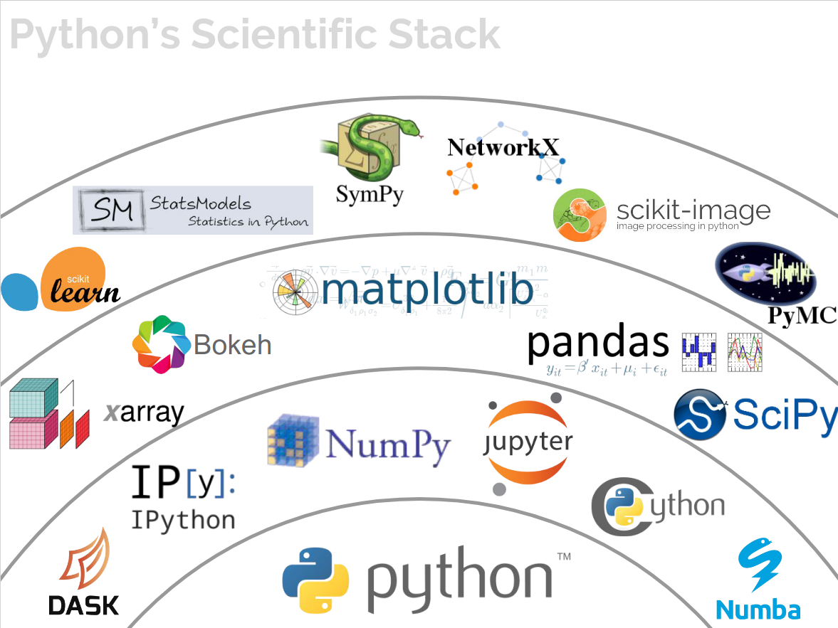
Python Ecosystem

So far, we have mostly used base Python
Important modules that facilitate working with Python in practice
- NumPy - handling arrays and linear algebra
- pandas - data frames
- matplotlib - visualization

Python Ecosystem

Source: Jake VanderPlas (PyCon, 2017)

NumPy

NumPy (Numerical Python) is a module for handling arrays
It provides various mathematical operations (linear algebra)
Example with base Python

Code

number_list = [1, 2, 3, 4, 5]
mean(number_list)

---------------------------------------------------------------------------
NameError                                 Traceback (most recent call last)
Cell In[73], line 2
      1 number_list = [1, 2, 3, 4, 5]
----> 2 mean(number_list)

NameError: name 'mean' is not defined

Code

mean_list = sum(number_list)/len(number_list)
print(mean_list)

3.0

NumPy

Example with NumPy

Code

import numpy as np
array = np.array([1, 2, 3, 4, 5])
mean_array = array.mean()
print(mean_array)

3.0

Why Use NumPy?

Python’s lists can be slow to process - substantial speed improvement possible using arrays
NumPys array object (ndarray) provides many supporting functions
Arrays (and NumPy) are very common in data science

NumPy Basics

Get Started with NumPy

Installation (not required in Anaconda)

# With UV (recommended)
uv add numpy

# With conda/pip (traditional)
conda install numpy
pip install numpy

After successful installation, import numpy (usually using the alias np)

Code

import numpy as np

Get Started with NumPy

We can initialize a ndarray from lists, tuples or array-like objects

Code

array = np.array([1, 2, 3, 4])
print(array)

[1 2 3 4]

Code

array_from_tuple = np.array((4, 3, 2, 1))
print(array_from_tuple)

[4 3 2 1]

Code

array_from_nestedlist = np.array([[1,2], [2, 3]])
print(array_from_nestedlist)

[[1 2]
 [2 3]]

Print class of array

Code

print(type(array))

<class 'numpy.ndarray'>

Array Dimensions

0-D arrays - scalars

Code

array_0d = np.array(3.14)
print(array_0d)

3.14

1-D arrays - vectors

Code

array_1d = np.array([1, 2, 3, 42])
print(array_1d)

[ 1  2  3 42]

2-D arrays - matrices / 2nd-order tensors

Code

array_2d = np.array([[1, 2, 3], [4, 5, 6]])
print(array_2d)

[[1 2 3]
 [4 5 6]]

Array Dimensions

3-D arrays - arrays / 3rd-order tensors

Code

array_3d = np.array([[[1, 2, 3], [4, 5, 6]],
                     [[1, 2, 3], [4, 5, 6]]])
print(array_3d)

[[[1 2 3]
  [4 5 6]]

 [[1 2 3]
  [4 5 6]]]

Higher-dimensional arrays: You can provide the number of dimensions during initialization

Code

array_5d = np.array([1, 2, 3, 4], ndmin=5)

print(array_5d)

[[[[[1 2 3 4]]]]]

Array Dimensions

Print the number of dimensions as well as the shape of the array

Code

print(array_0d.ndim)
print(array_1d.ndim)
print(array_2d.ndim)
print(array_3d.ndim)

Code

print(array_0d.shape)
print(array_1d.shape)
print(array_2d.shape)
print(array_3d.shape)

()
(4,)
(2, 3)
(2, 2, 3)

Array Elements

Access elements of arrays through its index number

Code

print(array_1d[0])
print(array_1d[-1])

1
42

Code

# Entry in 2nd row, 1st column
print(array_2d[1, 0])

Slicing Arrays

Arrays can be sliced in the same way as we sliced lists, i.e., using [start:end:step].

Code

print(array_2d[1, :])
print(array_3d[0, 0, :2])
print(array_1d[-3:-1])
print(array_5d[0,0,0,0,::2])

[4 5 6]
[1 2]
[2 3]
[1 3]

NumPy and Data Types

NumPy provides some additional data types. A character refers to the type of data, for example i to an interger
- b - boolean,
- f - float,
- S - string
- \(\ldots\)
Check data type of array calling .dtype

Code

print(array_1d.dtype)

int64

Code

array_str = np.array(["a", "b", "c"])
type(array_str.dtype)

numpy.dtypes.StrDType

NumPy and Data Types

You can provide the data type when you create a new array

Code

array_dt = np.array([1, 2, 3], dtype = 'S')

print(array_dt)
print(array_dt.dtype)

[b'1' b'2' b'3']
|S1

Change data type for existing array using .astype().

Reshaping Arrays

We can change the shape of an array
Reshape a 1-D array to a 2-D array

Code

print(array_1d)
array_1d2d = array_1d.reshape(2,2)

[ 1  2  3 42]

Code

print(array_1d2d)
print(array_1d2d.shape)

[[ 1  2]
 [ 3 42]]
(2, 2)

To reshape an array, the elements required for reshaping must be equal for both shapes (i.e., we cannot reshape a 1-D array with 8 elements to a 2-D array with 3 elements and 3 rows)

Reshaping Arrays

It’s possible to have one unknown dimension, i.e., we do not have to fully specify all dimensions. Use -1 in .reshape().

Code

array_2d_reshaped = array_2d.reshape(3,-1)
print(array_2d_reshaped)
print(array_2d_reshaped.shape)

[[1 2]
 [3 4]
 [5 6]]
(3, 2)

Flattening Arrays

Flattening \(=\) converting multidimensional array into 1-D array

Code

array_5d_flat = array_5d.reshape(-1)
print(array_5d_flat)

[1 2 3 4]

NumPy and Iteration

for-loop for 1-D arrays

Code

for a in array_1d:
    print(a)

for-loop for 2-D arrays and higher

Code

for a in array_2d:
    print(a)

[1 2 3]
[4 5 6]

Code

for a in array_2d:
    for x in a:
        print(x)

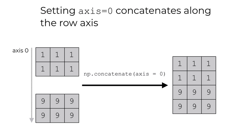
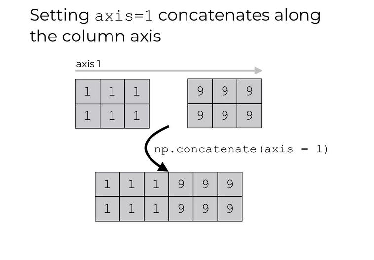
Joining Arrays

Joining \(=\) merging two or more arrays in a single array
In NumPy, we use concatenate to join arrays based on axes
axis argument indicates along which dimension arrays should be joined, axis = 0 along rows, axis = 1 along columns

Joining Arrays

Axis = 0
Axis = 1

Code

array_2d_2 = np.array([[0, 0, 1], [1, 0, 0]])
array_2d_join_axis0 = np.concatenate((array_2d, array_2d_2), axis = 0)
print(array_2d_join_axis0)

[[1 2 3]
 [4 5 6]
 [0 0 1]
 [1 0 0]]

Code

array_2d_join_axis1 = np.concatenate((array_2d, array_2d_2), axis = 1)
print(array_2d_join_axis1)

[[1 2 3 0 0 1]
 [4 5 6 1 0 0]]

Joining Arrays using Stack Functions

stack() is basically the same as concatenate(), except that it is done along a new axis

Axis = 0
Axis = 1

Code

array_join_axis0 = np.stack((array_1d, array_5d_flat), axis = 0)
print(array_join_axis0)

[[ 1  2  3 42]
 [ 1  2  3  4]]

Code

array_join_axis1 = np.stack((array_1d, array_5d_flat), axis = 1)
print(array_join_axis1)

[[ 1  1]
 [ 2  2]
 [ 3  3]
 [42  4]]

It’s possible to use the helpers hstack() and vstack() instead.

More Methods for Arrays

Splitting
- Joining \(=\) merge multiple arrays into one
- Splitting \(=\) split one array into multiple
- array_split(ary, indices_or_sections, axis=0)
- hsplit(), vsplit()
Searching for certain values
- where()
- searchsorted()
Sorting
- sort() (returns copy!)

More Methods for Arrays

Filter / masking
- Use booleans

Code

x = [True, False, True, False]
array_1d_filter = array_1d[x]
print(array_1d_filter)

[1 3]

Create a filter directly from array

Code

array_5d_filter = array_5d_flat[array_5d_flat > 2]
print(array_5d_filter)

[3 4]

ufuncs

NumPy provides ufuncs (Universal Functions) that work with ndarray objects \(\Rightarrow\) Speed up calculations (vectorization)

Code

# Add elements of 2 lists (item by item)
x = np.array([0, 0, 1, 10])
y = np.array([10, 0, 11, 123])
z = np.add(x, y)
print(z)

[ 10   0  12 133]

Code

# See if a function is a ufunc
print(type(np.add))

<class 'numpy.ufunc'>

Arithmetics

Operation	Function
`+`	`np.add()`
`-`	`np.substract()`
`*`	`np.multiply()`
`/`	`np.divide()`
`**`	`np.power()`
`%`	`np.mod()`
\(\ldots\)	\(\ldots\)

Linear Algebra with NumPy

Linear Algebra

Linear algebra is used in many algorithmic problems
Element-by-element operations

Code

print(x * 2)
print(y - 3)

[ 0  0  2 20]
[  7  -3   8 120]

Broadcasting
- Perform operations between arrays of different shapes

Code

a = np.array([[0,1], [2,3], [4,5]])
b = np.array([10, 100])
print(a*b)

[[  0 100]
 [ 20 300]
 [ 40 500]]

Linear Algebra

Dot product

Code

print(np.dot(x,y))

Linear Algebra

Identity matrix

Code

I3 = np.identity(3, dtype = int)
print(I3)

[[1 0 0]
 [0 1 0]
 [0 0 1]]

Matrix multiplication

Code

A = np.array([[1, 2, 3], [4, 5, 6]])
B = np.array([[2, 2], [1, 1], [3,3]])
C = np.matmul(A, B)
print(C)

[[13 13]
 [31 31]]

Linear Algebra

Transpose

Code

print(A.T)

[[1 4]
 [2 5]
 [3 6]]

Data Frames with Pandas

pandas

pandas is a Python module that helps to handle data in an easy and intuitive way
It provides data structures that are very useful if you work with real-world data in Python
pandas can be used to handle
- tabular data (think of an excel spreadsheet)
- time series data
- matrix data (organized in rows and columns)
- observational / statistical data sets

pandas

pandas is built on top of NumPy for a good integration with scientific computation
pandas is very good in terms of
- handling missing values
- data manipulation (e.g., inserting or deleting columns)
- data aligment with a set of labels (manually or automatic)
- data handling (data transformation and aggregation)
- converting data (e.g., to NumPy)
- advanced processing (indexing, slicing, subsetting)
- data loading and export
- speed

Data Structures in pandas

pandas builds on two basic data structures
- Series - 1-dimensional data, like a vector / one-dimensional array
- DataFrame - 2-dimensional data, tabular data in rows and columns
DataFrame
- \(=\) container of Series (which in turn are containers of int, str, \(\ldots\))
- organized in terms of an index (\(\sim\) rows) and columns

Getting Started with `pandas`

Install pandas

# With UV (recommended)
uv add pandas

# With conda/pip (traditional)
conda install pandas
pip install pandas

Load pandas, common alias pd (we’ll also load NumPy)

Code

import pandas as pd
import numpy as np

Creating Objects

Create a `Series` object

From a list

Code

s = pd.Series([1, 2, 3, np.nan, 6, 8])
print(s)

0    1.0
1    2.0
2    3.0
3    NaN
4    6.0
5    8.0
dtype: float64

Provide an index (\(\rightarrow\) row names)

Code

s = pd.Series([1, 2, 3, np.nan, 6, 8],
            index = ["a", "b", "c", "d", "e", "f"])
print(s)

a    1.0
b    2.0
c    3.0
d    NaN
e    6.0
f    8.0
dtype: float64

Creating Objects

Create a `Series` object

From a dictionary

Code

d = {'a': 1, 'b': 2, 'c': 3}
s = pd.Series(d)
print(s)

a    1
b    2
c    3
dtype: int64

Index values taken from dictionary d, hence index argument has no effect
- Series is first build from the dictionary and then reindexed –> NaN as result.

Code

d = {'a': 1, 'b': 2, 'c': 3}
s = pd.Series(d, index = ["x", "y", "z"])
print(s)

x   NaN
y   NaN
z   NaN
dtype: float64

Creating Objects

Create a `Series` object

Reindex a Series with Series.reindex(). Can you see what happens here?

Code

pd.Series(d).reindex(['a', 'x', 'y', 'b'], fill_value=np.nan)

a    1.0
x    NaN
y    NaN
b    2.0
dtype: float64

Creating Objects

Create a `DataFrame` object

From a dictionary

Code

data = {'col_1': [3, 2, 1, 0], 'col_2': ['a', 'b', 'c', 'd']}
df = pd.DataFrame.from_dict(data)
df

	col_1	col_2
0	3	a
1	2	b
2	1	c
3	0	d

Creating Objects

Create a `DataFrame` object

From a dictionary, providing an orientation

Code

data = {'row_1': [3, 2, 1, 0], 'row_2': [1, 2, 2, 3]}
df = pd.DataFrame.from_dict(data, orient='index')
df

	0	1	2	3
row_1	3	2	1	0
row_2	1	2	2	3

Creating Objects

Create a `DataFrame` object

From a NumPy array

Code

np.random.seed(3141)
dates = pd.date_range(start='2022-04-01', end='2022-04-06')
df = pd.DataFrame(np.random.randn(6, 4),
                index=dates, columns=['A', 'B', 'C', 'D'])
df

	A	B	C	D
2022-04-01	0.227769	-0.755529	1.144946	-0.352005
2022-04-02	-0.482710	0.655263	0.632421	-0.622162
2022-04-03	-0.143393	0.871788	0.332175	0.591673
2022-04-04	-2.419224	0.254834	-1.100392	-0.307889
2022-04-05	1.465222	-0.118808	0.329490	0.774558
2022-04-06	-0.079353	0.772174	-0.178963	0.195591

View Data

First and last rows using .head() and .tail(), respectively

Code

print(df.head(3))
print(df.tail(2))

                   A         B         C         D
2022-04-01  0.227769 -0.755529  1.144946 -0.352005
2022-04-02 -0.482710  0.655263  0.632421 -0.622162
2022-04-03 -0.143393  0.871788  0.332175  0.591673
                   A         B         C         D
2022-04-05  1.465222 -0.118808  0.329490  0.774558
2022-04-06 -0.079353  0.772174 -0.178963  0.195591

Show index

Code

print(df.index)

DatetimeIndex(['2022-04-01', '2022-04-02', '2022-04-03', '2022-04-04',
               '2022-04-05', '2022-04-06'],
              dtype='datetime64[us]', freq='D')

Array and Summary Statistics

Export as NumPy array (recommended)

Code

df_np = df.to_numpy()
print(df_np)
print(type(df_np))

[[ 0.22776912 -0.75552917  1.14494597 -0.35200459]
 [-0.48271037  0.65526347  0.63242091 -0.62216216]
 [-0.1433934   0.87178817  0.33217522  0.5916732 ]
 [-2.41922433  0.25483371 -1.10039219 -0.30788933]
 [ 1.46522216 -0.1188076   0.32948986  0.77455794]
 [-0.07935271  0.77217429 -0.17896296  0.19559059]]
<class 'numpy.ndarray'>

Similar result

Code

print(df.values)
print(type(df.values))

[[ 0.22776912 -0.75552917  1.14494597 -0.35200459]
 [-0.48271037  0.65526347  0.63242091 -0.62216216]
 [-0.1433934   0.87178817  0.33217522  0.5916732 ]
 [-2.41922433  0.25483371 -1.10039219 -0.30788933]
 [ 1.46522216 -0.1188076   0.32948986  0.77455794]
 [-0.07935271  0.77217429 -0.17896296  0.19559059]]
<class 'numpy.ndarray'>

Array and Summary Statistics

Summary statistics

Code

df.describe()

	A	B	C	D
count	6.000000	6.000000	6.000000	6.000000
mean	-0.238615	0.279954	0.193279	0.046628
std	1.262509	0.626941	0.767921	0.562320
min	-2.419224	-0.755529	-1.100392	-0.622162
25%	-0.397881	-0.025397	-0.051850	-0.340976
50%	-0.111373	0.455049	0.330833	-0.056149
75%	0.150989	0.742947	0.557359	0.492653
max	1.465222	0.871788	1.144946	0.774558

References

Downey, Allen. 2012. Think Python. " O’Reilly Media, Inc.".

Porter, Leo, and Daniel Zingaro. 2024. Learn AI-Assisted Python Programming: With Github Copilot and ChatGPT. Simon; Schuster.

Wentworth, Peter, Jeffrey Elkner, Allen B Downey, and Chris Meyer. 2015. “How to Think Like a Computer Scientist: Learning with Python 3.” Capı́tol.