# Original shapeprint(f"Original: {starwars.shape}")# Remove any row with missing valuesstarwars_complete = starwars.dropna()print(f"After dropna(): {starwars_complete.shape}")# Too aggressive! We lost most data (87 → 29 rows)
Original: (87, 14)
After dropna(): (6, 14)
Warning
Dropping all rows with any missing value is often too aggressive!
Handling Missing Values
Selective Removal
Drop rows only if specific columns are missing:
# Only drop if height or mass is missingstarwars_height_mass = starwars.dropna(subset=['height', 'mass'])print(f"Dropping rows with missing height or mass: {starwars_height_mass.shape}")# Much better! (87 → 59 rows)
Dropping rows with missing height or mass: (59, 14)
Handling Missing Values
Imputation: Filling Missing Values
Replace missing values with estimates:
# Create a copy for imputationstarwars_imputed = starwars.copy()# Fill missing height with medianmedian_height = starwars_imputed['height'].median()starwars_imputed['height'] = starwars_imputed['height'].fillna(median_height)# Fill missing mass with medianmedian_mass = starwars_imputed['mass'].median()starwars_imputed['mass'] = starwars_imputed['mass'].fillna(median_mass)# Check resultsprint(f"Missing height after imputation: {starwars_imputed['height'].isnull().sum()}")print(f"Missing mass after imputation: {starwars_imputed['mass'].isnull().sum()}")
Missing height after imputation: 0
Missing mass after imputation: 0
Checking for Duplicates
Identifying Duplicate Rows
# Check for duplicate rowsn_duplicates = starwars.duplicated().sum()print(f"Number of duplicate rows: {n_duplicates}")# Check for duplicate names (should each be unique)duplicate_names = starwars[starwars.duplicated(subset=['name'], keep=False)]print(f"\nDuplicate names: {len(duplicate_names)}")
Number of duplicate rows: 0

Duplicate names: 0
No duplicates found - this is a clean dataset!
Data Manipulation: Selection and Filtering
Selecting Columns
Choose Specific Columns
# Select single column (returns Series)names = starwars['name']print(f"Type: {type(names)}")print(names.head())
Type: <class 'pandas.core.series.Series'>
0    Luke Skywalker
1             C-3PO
2             R2-D2
3       Darth Vader
4       Leia Organa
Name: name, dtype: object
# Humans or Droidshumans_or_droids = starwars[(starwars['species'] =='Human') | (starwars['species'] =='Droid')]print(f"Humans or Droids: {len(humans_or_droids)}")humans_or_droids[['name', 'species']].head()
Humans or Droids: 41
name
species
0
Luke Skywalker
Human
1
C-3PO
Droid
2
R2-D2
Droid
3
Darth Vader
Human
4
Leia Organa
Human
Filtering Rows: Using Query
Alternative Syntax
The .query() method provides cleaner syntax:
# Same filter using querytall_humans_query = starwars.query('species == "Human" and height > 180')print(f"Tall humans (using query): {len(tall_humans_query)}")tall_humans_query[['name', 'height', 'species']].head()
Tall humans (using query): 15
name
height
species
3
Darth Vader
202.0
Human
8
Biggs Darklighter
183.0
Human
9
Obi-Wan Kenobi
182.0
Human
10
Anakin Skywalker
188.0
Human
20
Boba Fett
183.0
Human
Filtering with String Methods
String Contains
Code
# Find characters with "Skywalker" in their nameskywalkers = starwars[starwars['name'].str.contains('Skywalker', na=False)]skywalkers[['name', 'species', 'homeworld']]
name
species
homeworld
0
Luke Skywalker
Human
Tatooine
10
Anakin Skywalker
Human
Tatooine
41
Shmi Skywalker
Human
Tatooine
Filtering with String Methods
String Starts With
# Names starting with 'C'c_names = starwars[starwars['name'].str.startswith('C', na=False)]print(f"Characters whose name starts with 'C': {len(c_names)}")c_names[['name', 'species']].head()
Characters whose name starts with 'C': 5
name
species
1
C-3PO
Droid
12
Chewbacca
Wookiee
59
Cordé
NaN
60
Cliegg Lars
Human
86
Captain Phasma
Human
Data Manipulation: Sorting and Ranking
Sorting Data
Sort by Single Column
# Sort by height (ascending)sorted_by_height = starwars.sort_values('height')sorted_by_height[['name', 'height', 'species']].head()
# Sort by species (ascending) then height (descending)sorted_multi = starwars.sort_values(['species', 'height'], ascending=[True, False])sorted_multi[['name', 'species', 'height']].head(10)
name
species
height
45
Ratts Tyerel
Aleena
79.0
69
Dexter Jettster
Besalisk
198.0
50
Ki-Adi-Mundi
Cerean
198.0
57
Mas Amedda
Chagrian
196.0
68
Zam Wesell
Clawdite
168.0
21
IG-88
Droid
200.0
1
C-3PO
Droid
167.0
7
R5-D4
Droid
97.0
2
R2-D2
Droid
96.0
73
R4-P17
Droid
96.0
Data Manipulation: Creating New Variables
Adding New Columns
Simple Calculations
# Create a copy to work withsw = starwars.copy()# Convert height from cm to meterssw['height_m'] = sw['height'] /100sw[['name', 'height', 'height_m']].head()
# Group by species and countspecies_counts = starwars.groupby('species').size().sort_values(ascending=False)print("Top 10 species by count:")species_counts.head(5)
Top 10 species by count:
species
Human       35
Droid        6
Gungan       3
Kaminoan     2
Mirialan     2
dtype: int64
Aggregating Data
Summary Statistics by Group
# Average height and mass by speciesspecies_stats = starwars.groupby('species')[['height', 'mass']].mean()species_stats.sort_values('height', ascending=False).head(5)
# Count by species and genderspecies_gender = (starwars .groupby(['species', 'sex']) .size() .reset_index(name='count') .sort_values('count', ascending=False))species_gender.head(5)
species
sex
count
11
Human
male
26
10
Human
female
9
5
Droid
none
6
9
Gungan
male
3
18
Mirialan
female
2
Filtering After Grouping
Species with Multiple Characters
# Only species with at least 2 charactersspecies_multi = (starwars .groupby('species') .filter(lambda x: len(x) >=2) ['species'] .value_counts())print("Species with 2+ characters:")species_multi.head(5)
Species with 2+ characters:
species
Human      35
Droid       6
Gungan      3
Wookiee     2
Zabrak      2
Name: count, dtype: int64
Data Visualization
Introduction to Visualization
Why Visualize?
Patterns are easier to see than in tables
Outliers stand out visually
Distributions reveal data characteristics
Relationships between variables become clear
Essential for communication of results
Visualization Libraries in Python
Matplotlib: The foundational plotting library
Seaborn: Built on Matplotlib, easier for statistical plots
Distribution Plots: Histogram
Height Distribution
Code
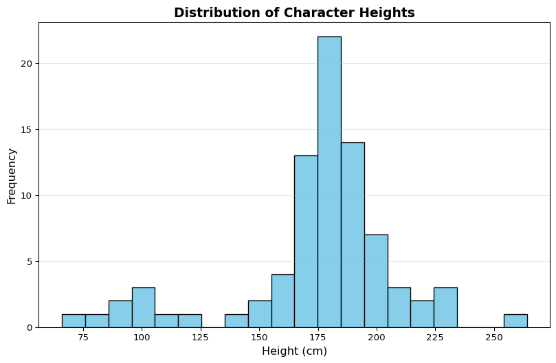
# Histogram of heightsimport matplotlib.pyplot as pltimport seaborn as snsplt.figure(figsize=(10, 6))plt.hist(starwars['height'].dropna(), bins=20, color='skyblue', edgecolor='black')plt.xlabel('Height (cm)', fontsize=12)plt.ylabel('Frequency', fontsize=12)plt.title('Distribution of Character Heights', fontsize=14, fontweight='bold')plt.grid(axis='y', alpha=0.3)plt.show()
Distribution Plots: Density Plot
Kernel Density Estimation
Code
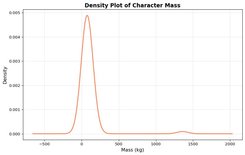
# Density plot of massplt.figure(figsize=(10, 6))starwars['mass'].dropna().plot(kind='density', color='coral', linewidth=2)plt.xlabel('Mass (kg)', fontsize=12)plt.ylabel('Density', fontsize=12)plt.title('Density Plot of Character Mass', fontsize=14, fontweight='bold')plt.grid(alpha=0.3)plt.show()
Box Plots: Comparing Distributions
Height by Gender
Code
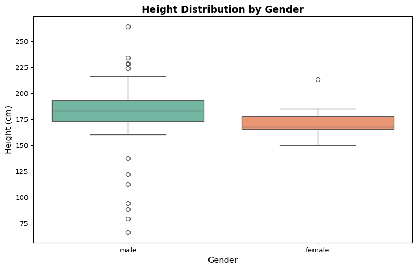
# Box plot: height by genderplt.figure(figsize=(10, 6))data_for_box = starwars[starwars['sex'].isin(['male', 'female'])].dropna(subset=['height', 'sex'])sns.boxplot(data=data_for_box, x='sex', y='height', palette='Set2')plt.xlabel('Gender', fontsize=12)plt.ylabel('Height (cm)', fontsize=12)plt.title('Height Distribution by Gender', fontsize=14, fontweight='bold')plt.show()
Box Plots: Identifying Outliers
Mass by Gender
Code
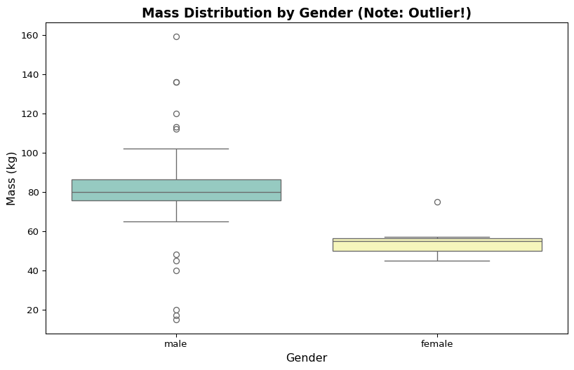
# Mass by gender - notice the outlier!plt.figure(figsize=(10, 6))data_mass = starwars[starwars['sex'].isin(['male', 'female'])].dropna(subset=['mass', 'sex'])sns.boxplot(data=data_mass, x='sex', y='mass', palette='Set3')plt.xlabel('Gender', fontsize=12)plt.ylabel('Mass (kg)', fontsize=12)plt.title('Mass Distribution by Gender (Note: Outlier!)', fontsize=14, fontweight='bold')plt.show()
Violin Plots: Density + Box Plot
Combining Information
Code
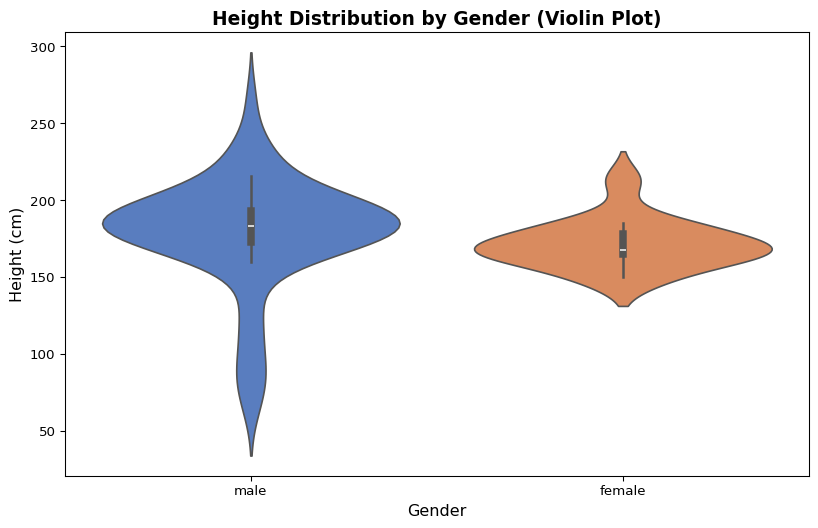
# Violin plot combines box plot and densityplt.figure(figsize=(10, 6))sns.violinplot(data=data_for_box, x='sex', y='height', palette='muted')plt.xlabel('Gender', fontsize=12)plt.ylabel('Height (cm)', fontsize=12)plt.title('Height Distribution by Gender (Violin Plot)', fontsize=14, fontweight='bold')plt.show()
Bar Plots: Categorical Counts
Species Distribution
Code
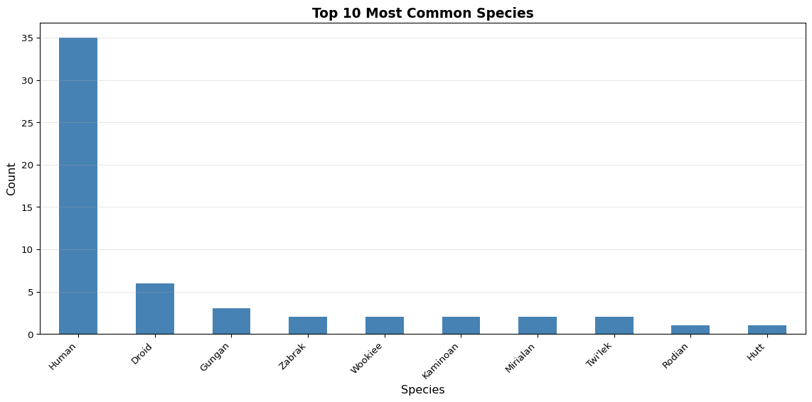
# Top 10 species by countplt.figure(figsize=(12, 6))top_species = starwars['species'].value_counts().head(10)top_species.plot(kind='bar', color='steelblue')plt.xlabel('Species', fontsize=12)plt.ylabel('Count', fontsize=12)plt.title('Top 10 Most Common Species', fontsize=14, fontweight='bold')plt.xticks(rotation=45, ha='right')plt.grid(axis='y', alpha=0.3)plt.tight_layout()plt.show()
Bar Plots: Grouped Bars
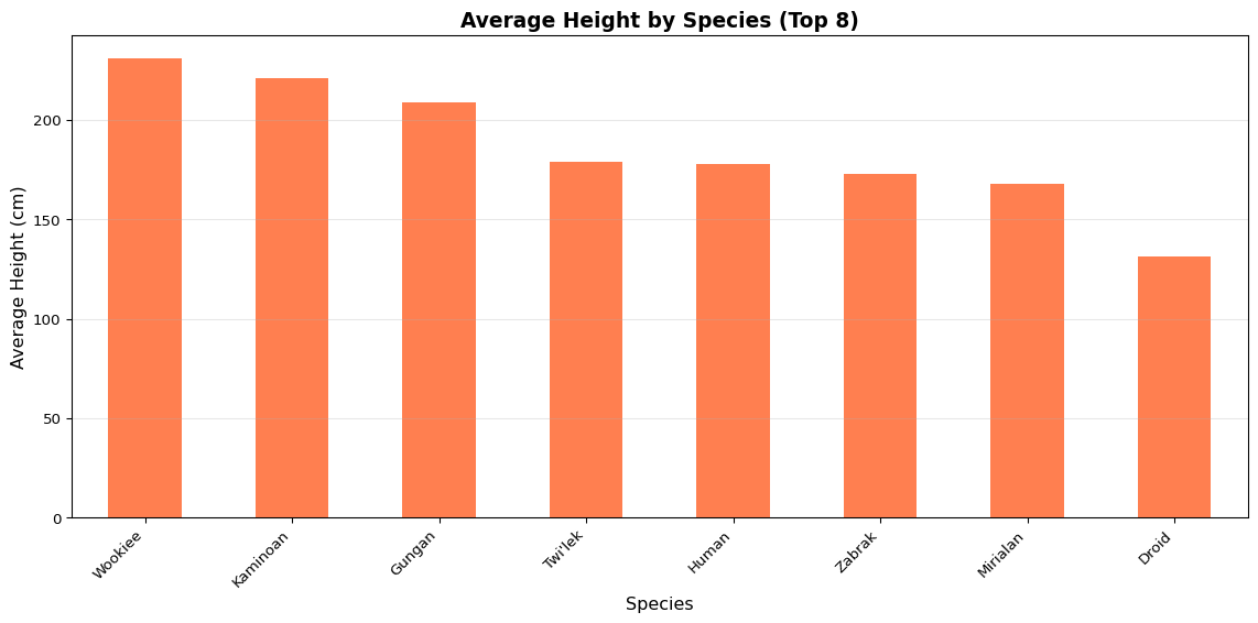
Average Height by Species
Code
# Average height for top speciesplt.figure(figsize=(12, 6))top_species_names = starwars['species'].value_counts().head(8).indexspecies_height = (starwars[starwars['species'].isin(top_species_names)] .groupby('species')['height'] .mean() .sort_values(ascending=False))species_height.plot(kind='bar', color='coral')plt.xlabel('Species', fontsize=12)plt.ylabel('Average Height (cm)', fontsize=12)plt.title('Average Height by Species (Top 8)', fontsize=14, fontweight='bold')plt.xticks(rotation=45, ha='right')plt.grid(axis='y', alpha=0.3)plt.tight_layout()plt.show()
Scatter Plots: Relationships
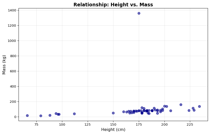
Height vs. Mass
Code
# Scatter plot: height vs massplt.figure(figsize=(10, 6))plt.scatter(starwars['height'], starwars['mass'], alpha=0.6, s=50, color='darkblue')plt.xlabel('Height (cm)', fontsize=12)plt.ylabel('Mass (kg)', fontsize=12)plt.title('Relationship: Height vs. Mass', fontsize=14, fontweight='bold')plt.grid(alpha=0.3)plt.show()
Scatter Plots: With Categories
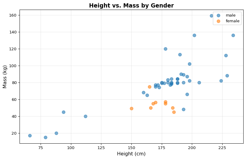
Colored by Gender
Code
# Scatter plot colored by genderplt.figure(figsize=(10, 6))data_scatter = starwars.dropna(subset=['height', 'mass', 'sex'])data_scatter = data_scatter[data_scatter['sex'].isin(['male', 'female'])]for gender in ['male', 'female']: subset = data_scatter[data_scatter['sex'] == gender] plt.scatter(subset['height'], subset['mass'], label=gender, alpha=0.6, s=60)plt.xlabel('Height (cm)', fontsize=12)plt.ylabel('Mass (kg)', fontsize=12)plt.title('Height vs. Mass by Gender', fontsize=14, fontweight='bold')plt.legend()plt.grid(alpha=0.3)plt.show()
Scatter Plots: With Regression Line
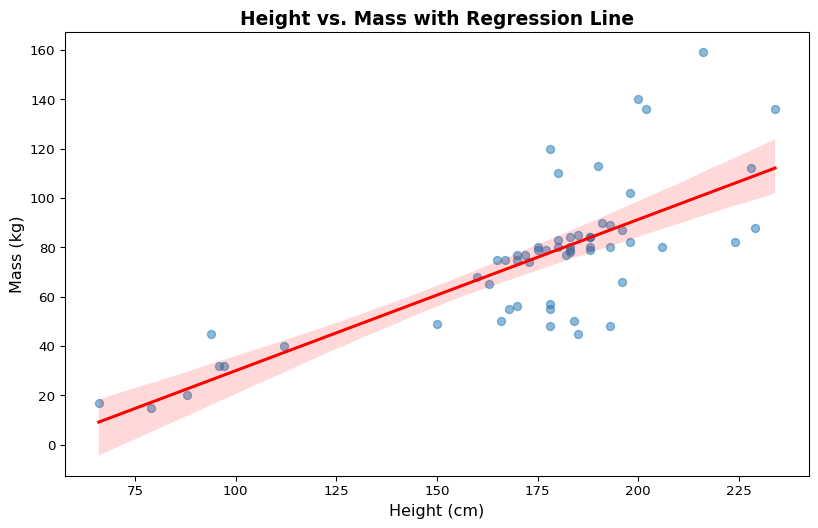
Adding Trend Line
Code
# Scatter with regression lineplt.figure(figsize=(10, 6))data_clean = starwars.dropna(subset=['height', 'mass'])# Remove extreme outlierdata_clean = data_clean[data_clean['mass'] <500]sns.regplot(data=data_clean, x='height', y='mass', scatter_kws={'alpha': 0.5}, line_kws={'color': 'red'})plt.xlabel('Height (cm)', fontsize=12)plt.ylabel('Mass (kg)', fontsize=12)plt.title('Height vs. Mass with Regression Line', fontsize=14, fontweight='bold')plt.show()
Correlation ≠ Causation (but it does waggle its eyebrows suggestively)
Just because height and mass correlate doesn’t mean being tall causes you to be heavy. Could be: - The other way around - Both caused by genetics? - Diet? The Force? 🤔
Sometimes we need to reshape data from wide to long format:
Code
# Create a simple wide dataset for demonstrationwide_data = pd.DataFrame({'character': ['Luke', 'Leia', 'Han'],'height': [172, 150, 180],'mass': [77, 49, 80]})print("Wide format:")print(wide_data)# Melt to long formatlong_data = wide_data.melt(id_vars='character', var_name='measurement', value_name='value')print("\nLong format:")print(long_data)
Wide format:
  character  height  mass
0      Luke     172    77
1      Leia     150    49
2       Han     180    80

Long format:
  character measurement  value
0      Luke      height    172
1      Leia      height    150
2       Han      height    180
3      Luke        mass     77
4      Leia        mass     49
5       Han        mass     80
Data Reshaping: Long to Wide
Pivoting Data
Code
# Pivot back to wide formatwide_again = long_data.pivot(index='character', columns='measurement', values='value')print("Back to wide format:")print(wide_again.reset_index())
Back to wide format:
measurement character  height  mass
0                 Han     180    80
1                Leia     150    49
2                Luke     172    77
Let’s analyze character names using text mining techniques:
Code
from sklearn.feature_extraction.text import CountVectorizer, TfidfVectorizerfrom collections import Counter# Analyze character names - extract all wordsall_names =' '.join(starwars['name'].dropna().values)words = all_names.lower().split()# Most common words in character namesword_counts = Counter(words)print("Most common words in Star Wars character names:")for word, count in word_counts.most_common(10):print(f" {word}: {count}")
Most common words in Star Wars character names:
  skywalker: 3
  lars: 3
  darth: 2
  organa: 2
  antilles: 2
  fett: 2
  jar: 2
  luke: 1
  c-3po: 1
  r2-d2: 1
Text Feature Engineering
Creating Text-Based Features
Code
# Extract features from text datasw_text = starwars.copy()# Has title (Master, Darth, etc.)sw_text['has_title'] = sw_text['name'].str.contains('Master|Darth|Captain|Admiral|General', case=False, na=False)# Number of words in namesw_text['name_words'] = sw_text['name'].str.split().str.len()# Starts with vowelsw_text['starts_vowel'] = sw_text['name'].str[0].str.lower().isin(['a', 'e', 'i', 'o', 'u'])# Show examplessw_text[['name', 'has_title', 'name_words', 'starts_vowel']].head(10)
name
has_title
name_words
starts_vowel
0
Luke Skywalker
False
2
False
1
C-3PO
False
1
False
2
R2-D2
False
1
False
3
Darth Vader
True
2
False
4
Leia Organa
False
2
False
5
Owen Lars
False
2
True
6
Beru Whitesun Lars
False
3
False
7
R5-D4
False
1
False
8
Biggs Darklighter
False
2
False
9
Obi-Wan Kenobi
False
2
True
N-gram Analysis
Character-Level Patterns
Code
# Analyze character patterns in namesfrom collections import defaultdictdef get_bigrams(text):"""Extract character bigrams from text"""return [text[i:i+2] for i inrange(len(text)-1)]# Get all character bigrams from namesall_bigrams = []for name in starwars['name'].dropna(): all_bigrams.extend(get_bigrams(name.lower().replace(' ', '')))bigram_counts = Counter(all_bigrams)print("Most common character bigrams in names:")for bigram, count in bigram_counts.most_common(15):print(f" '{bigram}': {count}")
Most common character bigrams in names:
  'ar': 20
  'an': 14
  'in': 13
  'er': 11
  'or': 11
  'es': 9
  'al': 9
  'na': 8
  'wa': 7
  'da': 7
  'la': 7
  'un': 7
  'ta': 7
  'ba': 7
  're': 7
Text Similarity Analysis
Finding Similar Character Names
Code
from sklearn.feature_extraction.text import TfidfVectorizerfrom sklearn.metrics.pairwise import cosine_similarity# Create TF-IDF vectors from character namesnames_clean = starwars['name'].dropna()vectorizer = TfidfVectorizer(analyzer='char', ngram_range=(2,3))name_vectors = vectorizer.fit_transform(names_clean)# Calculate similarity matrixsimilarity_matrix = cosine_similarity(name_vectors)# Find most similar name pairsdef find_similar_names(names, sim_matrix, top_n=5): results = []for i inrange(len(names)):for j inrange(i+1, len(names)): sim = sim_matrix[i, j]if sim >0.3: # Threshold for similarity results.append((names.iloc[i], names.iloc[j], sim)) results.sort(key=lambda x: x[2], reverse=True)return results[:top_n]similar = find_similar_names(names_clean, similarity_matrix)print("Most similar character name pairs:")for name1, name2, score in similar:print(f" {name1} <-> {name2}: {score:.3f}")
Most similar character name pairs:
  Luke Skywalker <-> Shmi Skywalker: 0.627
  Luke Skywalker <-> Anakin Skywalker: 0.615
  Anakin Skywalker <-> Shmi Skywalker: 0.601
  Wedge Antilles <-> Raymus Antilles: 0.521
  Darth Vader <-> Darth Maul: 0.442
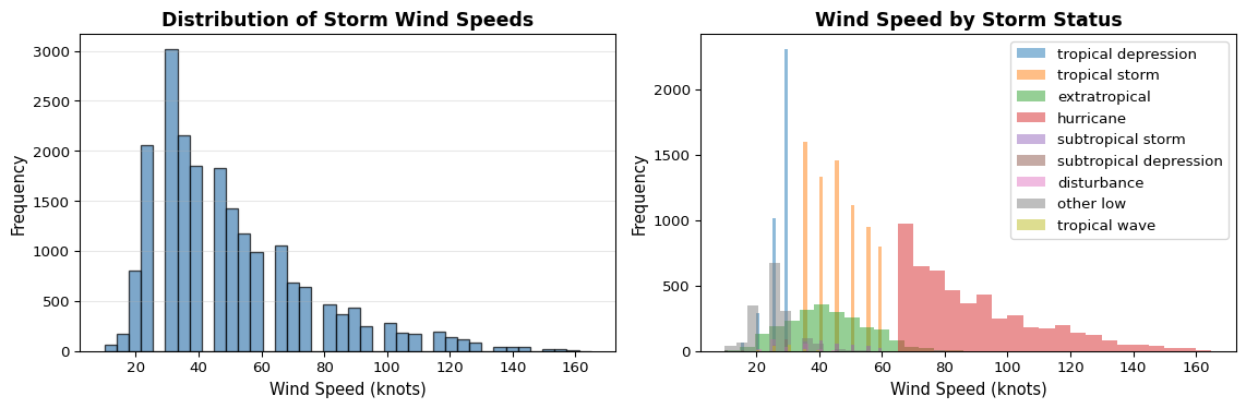
# Distribution of maximum wind speedsplt.figure(figsize=(12, 4))# Histogramplt.subplot(1, 2, 1)plt.hist(storms['wind'], bins=40, color='steelblue', edgecolor='black', alpha=0.7)plt.xlabel('Wind Speed (knots)', fontsize=11)plt.ylabel('Frequency', fontsize=11)plt.title('Distribution of Storm Wind Speeds', fontsize=13, fontweight='bold')plt.grid(axis='y', alpha=0.3)# By statusplt.subplot(1, 2, 2)for status in storms['status'].unique(): data = storms[storms['status'] == status]['wind'] plt.hist(data, bins=20, alpha=0.5, label=status)plt.xlabel('Wind Speed (knots)', fontsize=11)plt.ylabel('Frequency', fontsize=11)plt.title('Wind Speed by Storm Status', fontsize=13, fontweight='bold')plt.legend()plt.tight_layout()plt.show()
Temporal Trends
Storms Over Time
Code
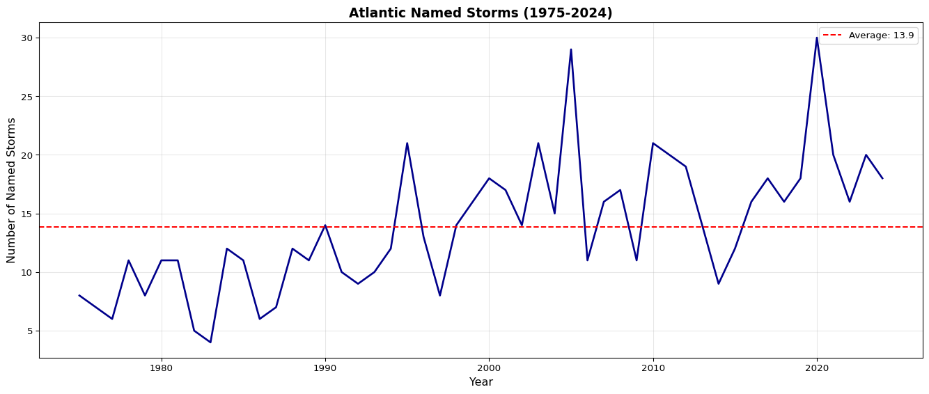
# Number of storms per yearstorms_per_year = storms.groupby(['year', 'name']).first().groupby('year').size()plt.figure(figsize=(14, 6))storms_per_year.plot(kind='line', linewidth=2, color='darkblue')plt.xlabel('Year', fontsize=12)plt.ylabel('Number of Named Storms', fontsize=12)plt.title('Atlantic Named Storms (1975-2024)', fontsize=14, fontweight='bold')plt.grid(alpha=0.3)plt.axhline(y=storms_per_year.mean(), color='red', linestyle='--', label=f'Average: {storms_per_year.mean():.1f}')plt.legend()plt.tight_layout()plt.show()
Interactive Geographic Visualization
Storm Tracks on Map
Code
# Select a few major storms for clear visualizationmajor_storms = ['Katrina', 'Sandy', 'Maria', 'Harvey', 'Irma']storms_major = storms[storms['name'].isin(major_storms)]# Create interactive map with storm tracksfig = px.scatter_geo(storms_major, lat='lat', lon='long', color='name', size='wind', hover_data=['status', 'wind', 'pressure', 'datetime'], title='Major Hurricane Tracks (Interactive Map)', projection='natural earth', template='plotly_white', width=1000, height=600)fig.update_geos( showcountries=True, showcoastlines=True, showland=True, fitbounds="locations", projection_scale=1.5)fig.show()
# Analyze hurricane trends by decadehurricanes_only = storms[storms['status'] =='hurricane'].copy()# Get maximum wind speed per stormmax_winds = (hurricanes_only .groupby(['name', 'year', 'decade']) ['wind'] .max() .reset_index())# Count by decadedecade_counts = max_winds.groupby('decade').size().reset_index(name='count')# Average maximum wind speed by decadedecade_intensity = max_winds.groupby('decade')['wind'].mean().reset_index()decade_intensity.columns = ['decade', 'avg_max_wind']print("Hurricanes per decade:")print(decade_counts)print("\n\nAverage maximum wind speed by decade:")print(decade_intensity)
Hurricanes per decade:
   decade  count
0    1970     27
1    1980     52
2    1990     64
3    2000     74
4    2010     72
5    2020     48


Average maximum wind speed by decade:
   decade  avg_max_wind
0    1970     92.777778
1    1980     90.000000
2    1990     93.984375
3    2000     98.445946
4    2010     96.458333
5    2020     99.062500
Visualization: Decadal Trends
Interactive Comparison
Code
# Merge for plottingdecade_stats = decade_counts.merge(decade_intensity, on='decade')# Create subplot with two y-axesfig = go.Figure()fig.add_trace(go.Bar( x=decade_stats['decade'], y=decade_stats['count'], name='Number of Hurricanes', marker_color='steelblue', yaxis='y', opacity=0.7))fig.add_trace(go.Scatter( x=decade_stats['decade'], y=decade_stats['avg_max_wind'], name='Avg Max Wind Speed', marker_color='red', mode='lines+markers', yaxis='y2', line=dict(width=3)))fig.update_layout( title='Hurricane Frequency and Intensity by Decade', xaxis=dict(title='Decade'), yaxis=dict(title='Number of Hurricanes', side='left'), yaxis2=dict(title='Average Max Wind Speed (knots)', side='right', overlaying='y'), template='plotly_white', width=1000, height=500, hovermode='x unified')fig.show()
Recent Trends: 2020s show increased storm frequency
Geographic Patterns: Most storms originate in tropical Atlantic, moving northwest
Major Storms: Katrina (2005), Sandy (2012), Maria (2017) were devastating
How Does This Relate to Climate Change?
Climate Impact Note
Data suggests increasing frequency of named storms in recent decades, consistent with climate change predictions.
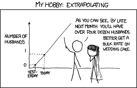
Important: We can responsibly discuss trends within our data range (1975-2020), but extrapolating far into the future requires climate models, not just historical data!
# Create hexbin density mapfig = px.density_mapbox(storms, lat='lat', lon='long', z='wind', # Weight by wind speed (intensity) radius=20, # Smooths out the points zoom=2.5, mapbox_style='carto-positron', # Cleaner background than open-street-map title='Storm Track & Intensity Density Heatmap', hover_name='name', # Show name on hover hover_data=['datetime'], # Show date on hover width=900, height=600, center=dict(lat=25, lon=-65), color_continuous_scale='Viridis', opacity=0.5)fig.show()
Tip
Interactive maps allow exploration of spatial patterns that static plots miss!
Best Practices and Tips
Data Handling Best Practices
Key Recommendations
Always explore data first: Use .head(), .info(), .describe()
Check for missing values: Decide on strategy (drop, impute, or keep)
Look for duplicates: Use .duplicated() to check
Understand data types: Ensure correct types for each column
Document your workflow: Comment your code, explain decisions
Data Handling Best Practices
More Recommendations
Create copies when modifying: Use .copy() to avoid unintended changes
Chain operations: Use method chaining for readable pipelines
Save intermediate results: Don’t lose work in long analyses
Validate results: Sanity check numbers and visualizations
Export clean data: Save processed data for reproducibility
Hofstadter’s Law - Data Science Edition
Mistakes to Watch For
SettingWithCopyWarning: Always use .copy() when creating subsets
Chained indexing: Use .loc[] instead of chained [][]
Ignoring missing values: Many operations silently exclude NaN
Wrong data types: Strings vs. numbers, dates as strings
Outliers affecting means: Use median for skewed distributions
Over-cleaning: Don’t remove too much data unnecessarily
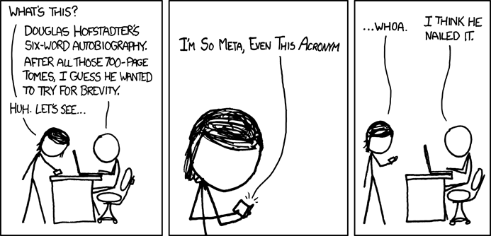
“Data cleaning always takes longer than you expect, even when you take into account Hofstadter’s Law.”