import numpy as np
import pandas as pd
import random
import matplotlib.pyplot as plt
#%matplotlib inline
#from matplotlib.pylab import rcParams
#rcParams['figure.figsize'] = 12, 10Statistical Programming: Problem Set 3 — Solutions
Exercise 1: Linear Regression: Prediction
We consider a regression problem where we want to predict our dependent variable \(Y\) in terms of the explanatory variable \(X\). In this exercise we try to create an optimal prediction of \(Y\) given \(X\).
Load the
predictiondata and assess its structure. Generate a scatter plot of the \(Y\) values against the \(X\) values.Run a linear regression using the
sklearnpackage and add the regression line to the scatter plot. Compute the in-sample MSE in prediction.Now load the
predictiontestdata set and assess how good your model predicts the new observations. Compute the out-of-sample MSE in prediction and illustrate your results in the scatter plot.Try to improve your predictive performance by including high-order polynomials of the variable \(X\) in your regression. Add the predictions from the polynomial model to the scatter plot.
Hint: Use the
sklearn.preprocessing.PolynomialFeaturesmodule to generate the polynomials.Increase the polynomial order in your approximation of the regression curve and see how the in-sample and out-of-sample MSE behave.
Generate a plot of the in-sample and out-of-sample MSE depending on the order of the polynomial, \(q\), in the regression function.
Solution to Exercise 1.1.
import csv
import pandas as pd
data = pd.read_csv(r"https://raw.githubusercontent.com/JanTeichertKluge/data-statprog/refs/heads/main/data/prediction.csv", sep=',', na_values=".")
data.head()| x | y | |
|---|---|---|
| 0 | 1.047198 | 9.242999 |
| 1 | 1.186824 | 6.861050 |
| 2 | 1.326450 | -2.258883 |
| 3 | 1.466077 | 3.645338 |
| 4 | 1.605703 | 5.755031 |
data.shape (49, 2)plt.figure(1,figsize=(15,5))
plt.plot(data['x'],data['y'],'.')
plt.show()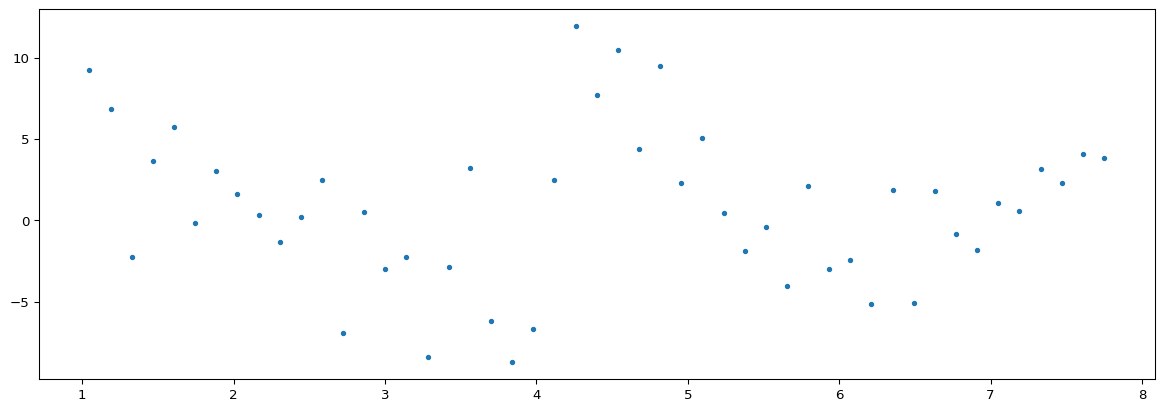
Solution to Exercise 1.2.
x = pd.DataFrame(data, columns=['x'])
y = pd.DataFrame(data, columns=['y'])
from sklearn.linear_model import LinearRegression
linmod = LinearRegression()
linmod.fit(x, y)
ypred_linmod = linmod.predict(x)plt.figure(1,figsize=(15,5))
plt.plot(data['x'],data['y'],'.')
plt.plot(data['x'], ypred_linmod)
plt.show()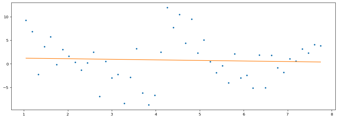
MSE_ins = np.mean((ypred_linmod - y)**2)

print("MSE (ins)", MSE_ins)
MSE (ins) 22.15966314172156Solution to Exercise 1.3.
import csv
import pandas as pd
datatest = pd.read_csv(r"https://raw.githubusercontent.com/JanTeichertKluge/data-statprog/refs/heads/main/data/predictiontest.csv", sep=',', na_values=".")
datatest.head()| xtest | ytest | |
|---|---|---|
| 0 | 1.047198 | 5.808596 |
| 1 | 1.186824 | 1.274230 |
| 2 | 1.326450 | 4.892476 |
| 3 | 1.466077 | -3.124069 |
| 4 | 1.605703 | 6.282259 |
# ensure that xtest and x have the same column names
datatest.rename(columns={'xtest': 'x',
                        'ytest': 'y'}, inplace=True)
xtest = pd.DataFrame(datatest, columns=['x'])
ytest = pd.DataFrame(datatest, columns=['y'])datatest.shape(49, 2)Generate out-of-sample predictions
y_linmod_oos = linmod.predict(xtest)plt.figure(1,figsize=(15,5))
#plt.plot(data['x'],data['y'],'.')
#plt.plot(data['x'], ypred_linmod)
plt.plot(datatest['x'], datatest['y'],'.', color = "red", label = "Test Data")
plt.plot(datatest['x'], y_linmod_oos,'.', color = "olive", label = "Predicted values")
plt.legend()
plt.show()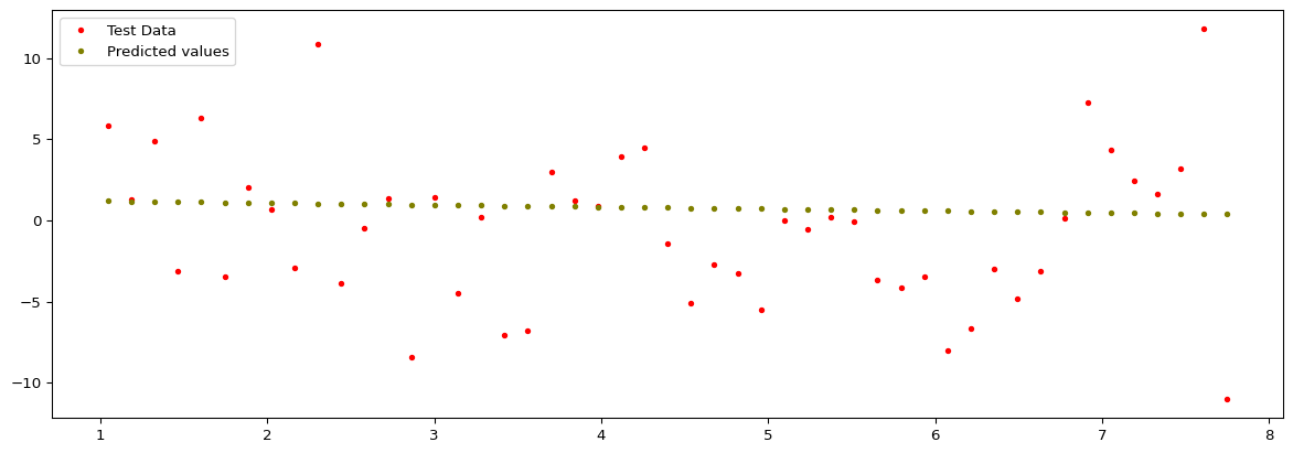
Compute the out-of-sample MSE in prediction.
# MSE
MSE = np.mean((y_linmod_oos - ytest)**2)

print("MSE basic linear Model: ", MSE)
MSE basic linear Model: 24.3254796898932Solution to Exercise 1.4.
from sklearn.preprocessing import PolynomialFeatures
poly_q = 5
x_t = PolynomialFeatures(poly_q, include_bias=False).fit_transform(x)
x_t = pd.DataFrame(x_t)
x_t.head()| 0 | 1 | 2 | 3 | 4 | |
|---|---|---|---|---|---|
| 0 | 1.047198 | 1.096623 | 1.148381 | 1.202581 | 1.259340 |
| 1 | 1.186824 | 1.408551 | 1.671702 | 1.984016 | 2.354677 |
| 2 | 1.326450 | 1.759470 | 2.333850 | 3.095735 | 4.106339 |
| 3 | 1.466077 | 2.149381 | 3.151156 | 4.619837 | 6.773034 |
| 4 | 1.605703 | 2.578282 | 4.139955 | 6.647537 | 10.673970 |
Fit the polynomial model.
polymod = LinearRegression()
polymod.fit(x_t, y)LinearRegression()In a Jupyter environment, please rerun this cell to show the HTML representation or trust the notebook.
On GitHub, the HTML representation is unable to render, please try loading this page with nbviewer.org.
Parameters
Generate in-sample and out-of-sample predictions and compute the in-sample and out-of-sample MSE.
# Generate transformation for the test sample
x_t_test = PolynomialFeatures(poly_q, include_bias=False).fit_transform(xtest)
y_poly_ins = polymod.predict(x_t)
y_poly_oos = polymod.predict(x_t_test)
MSE_poly_ins = np.mean((y_poly_ins - y)**2)
MSE_poly = np.mean((y_poly_oos - ytest)**2)
print("MSE polyn. Model (in sample): ", MSE_poly_ins)
print("MSE polyn. Model: ", MSE_poly)MSE polyn. Model (in sample): 16.334817378708188
MSE polyn. Model: 28.10115641312176# In sample predictions
plt.figure(1,figsize=(15,5))
#plt.plot(data['x'],data['y'],'.')
#plt.plot(data['x'], ypred_linmod)
plt.plot(data['x'], data['y'],'.', color = "red", label = "Train Data")
plt.plot(data['x'], ypred_linmod,'.', color = "olive", label = "Predicted values (Linear Mod.)")
plt.plot(data['x'], y_poly_ins, linestyle = "dotted", color = "blue", label = "Predicted values (Polynom. Model)")
plt.legend()
plt.show()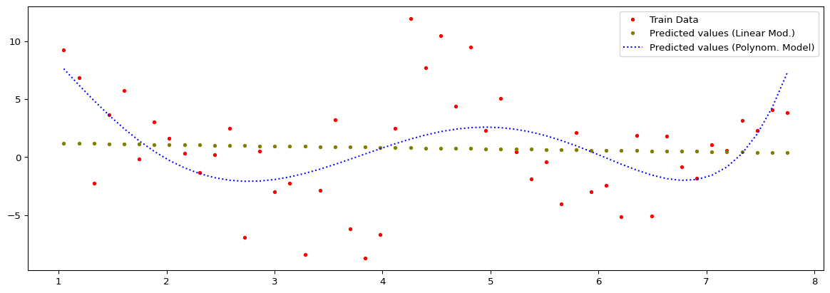
# Out of sample predictions

plt.figure(1,figsize=(15,5))
#plt.plot(data['x'],data['y'],'.')
#plt.plot(data['x'], ypred_linmod)
plt.plot(datatest['x'], datatest['y'],'.', color = "red", label = "Test Data")
plt.plot(datatest['x'], y_linmod_oos,'.', color = "olive", label = "Predicted values (Linear Mod.)")
plt.plot(datatest['x'], y_poly_oos, linestyle = "dotted", color = "blue", label = "Predicted values (Polynom. Model)")
plt.legend()
plt.show()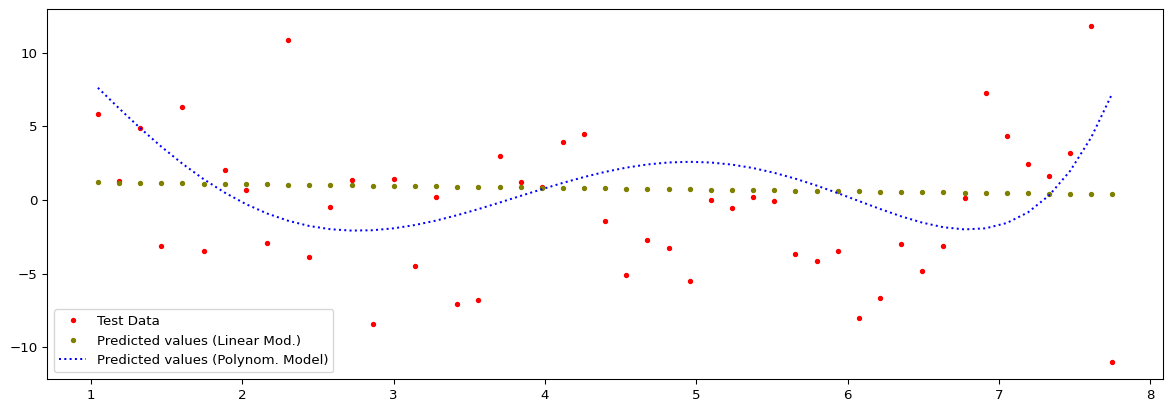
Solution to Exercise 1.5.
x_t_15 = PolynomialFeatures(15, include_bias=False).fit_transform(x)
x_t_15_test = PolynomialFeatures(15, include_bias=False).fit_transform(xtest)
polymod15 = LinearRegression()
polymod15.fit(x_t_15, y)
y_poly_15_ins = polymod15.predict(x_t_15)
y_poly_15_oos = polymod15.predict(x_t_15_test)
MSE_poly_15_ins = np.mean((y_poly_15_ins - y)**2)
MSE_poly_15 = np.mean((y_poly_15_oos - ytest)**2)
print("MSE polyn. Model (in sample): ", MSE_poly_15_ins)
print("MSE polyn. Model: ", MSE_poly_15)MSE polyn. Model (in sample): 9.978242828363555
MSE polyn. Model: 30.093810754859245# In sample predictions
plt.figure(1,figsize=(15,5))
plt.plot(data['x'],data['y'],'.')
plt.plot(data['x'], y_poly_15_ins)
plt.title("In Sample Predictions")
plt.show()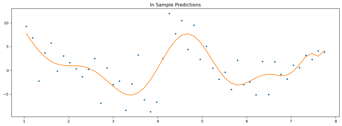
# Out of sample predictions

plt.figure(1,figsize=(15,5))
#plt.plot(data['x'],data['y'],'.')
#plt.plot(data['x'], ypred_linmod)
plt.plot(datatest['x'], datatest['y'],'.', color = "red", label = "Test Data")
plt.plot(datatest['x'], y_poly_15_oos, linestyle = "dotted", color = "blue", label = "Predicted values (Polynom. Model)")
plt.title("Out-of-Sample Predictions")
plt.legend()
plt.show()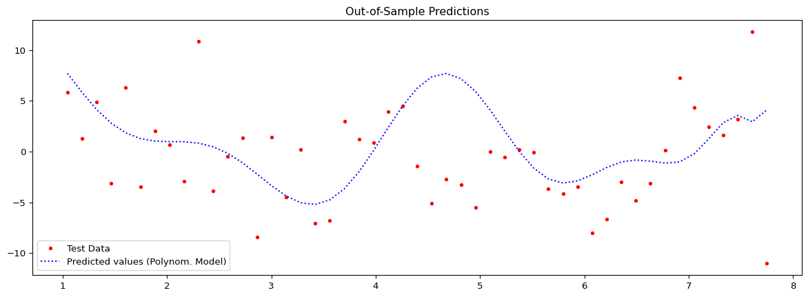
Solution to Exercise 1.6.
q = np.arange(1,12,1)
MSE_ins = np.zeros(len(q))
MSE_oos = np.zeros(len(q))

for i in range(0,len(q)):
    x_t = PolynomialFeatures(q[i], include_bias=False).fit_transform(x)
    x_t_test = PolynomialFeatures(q[i], include_bias=False).fit_transform(xtest)

    polymod = LinearRegression()
    polymod.fit(x_t, y)
    y_poly_ins = polymod.predict(x_t)
    y_poly_oos = polymod.predict(x_t_test)

    MSE_ins[i] = np.mean((y_poly_ins - y)**2)
    MSE_oos[i] = np.mean((y_poly_oos - ytest)**2)


print("MSE polyn. Model (in sample): ", MSE_ins)
print("MSE polyn. Model: ", MSE_oos)
MSE polyn. Model (in sample): [22.15966314 21.29031775 20.69472006 17.02803087 16.33481738 14.92459239
13.2774052 11.3904732 11.22843517 10.76808765 10.16711495]
MSE polyn. Model: [24.32547969 22.40355763 23.28305662 25.86654804 28.10115641 25.74330172
23.81919807 25.95598424 26.66503608 26.58432041 27.4645981 ]plt.figure(1,figsize=(15,5))
plt.plot(q, MSE_ins, label = "MSE in-sample")
plt.plot(q, MSE_oos, label = "MSE out-of-sample")
plt.legend()
plt.show()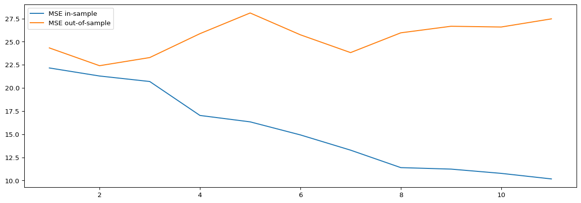
Exercise 2: Linear Regression: Inference I - Case Study Oregon Health Experiment
In this problem, we analyze a random subset from the Oregon Health Experiment Data. In this large-scale experiment, access to Medicaid (U.S. public health insurance) was provided randomly in a lottery. More information can be found here. The problem set is based on the published study by Finkelstein et al. (2012, Quarterly Journal of Economics).
Load the data and create a pandas data frame.
Our dependent variable is the number of doctor visits in the last 6 months (“docvis”). Inspect the data set and generate a frequency table for the outcome variable”docvis” as well as a barplot.
Hint: For the frequency table use
pd.crosstab.We are interested in estimating an intent-to-treatment effect, i.e. how does access to Medicaid increase the number of doctor visits. Thus, our regression model is \[ DOCVIS_i = \beta_0 + \beta_1 * TREATMENT_i + X_i'\beta + \varepsilon_i,\] where \(DOCVIS_i\) is the number of doctor visits, \(TREATMENT_i\) is access to health insurance. The controls \(X_i\) contain the variables:
dddraw_sur_2 ddddraw_sur_3 ddddraw_sur_4 ddddraw_sur_5 ddddraw_sur_6 ddddraw_sur_7 dddnumhh_li_2 dddnumhh_li_3 ddddraXnum_2_2 ddddraXnum_2_3 ddddraXnum_3_2 ddddraXnum_3_3 ddddraXnum_4_2 ddddraXnum_5_2 ddddraXnum_6_2 ddddraXnum_7_2
Hint: At the very end of this exercise, you’ll find the list with column names that you need to build your data frame.
Is there a significant effect of \(TREATMENT\), i.e., access to Medicaid?
Now, we would like to extend the model and include variables on gender, education and race/ethnicity in addition to the technical regressors
female_list, hhinc_pctfpl_12m, age2008, edu_12m_2, edu_12m_3, edu_12m_4, english_list, zip_msa, race_white_12m, race_black_12m, race_hisp_12m
How do you interpret the coefficients on female, age and income? Does your conclusion from part 2. change?
(optional) Does the treatment dummy vary with the observable characteristics? Run a regression that includes the interaction of the treatment variable with the non-technical regressors. Interpret your findings.
Hint: Use the formula interface of the
statsmodel.formula.apito generate interactions.How would you summarize your results? Are the OLS conditions met in the Oregon Health Example?
import numpy as npSolution to Exercise 2.1.
import csv
import pandas as pd
Oregdata = pd.read_csv(r"https://raw.githubusercontent.com/JanTeichertKluge/data-statprog/refs/heads/main/data/Oregon.csv", sep=',', na_values=".")
Oregdata.head()| household_id | treatment | english_list | female_list | zip_msa | weight_12m | docvis | hhinc_pctfpl_12m | race_hisp_12m | race_white_12m | ... | ddddraXnum_3_3 | ddddraXnum_4_2 | ddddraXnum_5_2 | ddddraXnum_6_2 | ddddraXnum_7_2 | edu_12m_2 | edu_12m_3 | edu_12m_4 | age2008 | chronicdis | |
|---|---|---|---|---|---|---|---|---|---|---|---|---|---|---|---|---|---|---|---|---|---|
| 0 | 100002 | 1 | 1 | 1 | 1 | 1.0 | 0 | 60.054909 | 0 | 1 | ... | 0 | 0 | 0 | 0 | 0 | 1 | 0 | 0 | 24 | 0 |
| 1 | 100005 | 1 | 0 | 1 | 1 | 1.0 | 0 | 129.710540 | 1 | 0 | ... | 0 | 0 | 0 | 0 | 0 | 1 | 0 | 0 | 39 | 1 |
| 2 | 100006 | 1 | 1 | 0 | 1 | 1.0 | 1 | 34.134354 | 0 | 1 | ... | 0 | 0 | 0 | 0 | 0 | 0 | 0 | 1 | 62 | 3 |
| 3 | 100009 | 0 | 1 | 1 | 1 | 1.0 | 1 | 47.788094 | 0 | 1 | ... | 0 | 0 | 0 | 0 | 0 | 1 | 0 | 0 | 31 | 0 |
| 4 | 100013 | 1 | 1 | 0 | 0 | 1.0 | 10 | 11.542013 | 0 | 1 | ... | 0 | 0 | 0 | 0 | 0 | 1 | 0 | 0 | 45 | 2 |
5 rows × 32 columns
Solution to Exercise 2.2.
docvis = pd.DataFrame(Oregdata, columns=['docvis'], dtype='int')
# docvis = Oregdata[['docvis']]
docvis = docvis.values[:]
#type(docvis)
import matplotlib.pyplot as plt
fig = plt.figure(figsize=(9, 4))
plt.hist(docvis, bins = 30, density=True,label='empirical density') # plotting a histogram
plt.show()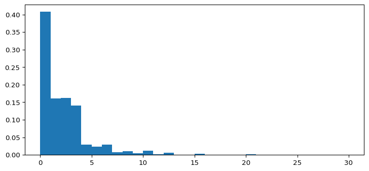
pd.crosstab(columns=Oregdata["docvis"], index="count")| docvis | 0 | 1 | 2 | 3 | 4 | 5 | 6 | 7 | 8 | 9 | ... | 16 | 17 | 18 | 19 | 20 | 22 | 24 | 25 | 27 | 30 |
|---|---|---|---|---|---|---|---|---|---|---|---|---|---|---|---|---|---|---|---|---|---|
| row_0 | |||||||||||||||||||||
| count | 6325 | 2505 | 2506 | 2190 | 459 | 363 | 446 | 106 | 169 | 58 | ... | 7 | 3 | 9 | 4 | 31 | 1 | 4 | 6 | 1 | 8 |
1 rows × 26 columns
(+) Boxplot.
fig = plt.subplots(1,1)[1]
fig.boxplot(docvis)
plt.show()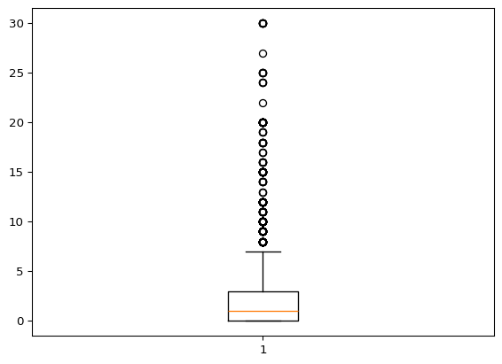
We are interested in estimating an intent-to-treatment effect, i.e. how does access to Medicaid increase the number of doctor visits. Thus, our regression model is
\[ DOCVIS_i = \beta_0 + \beta_1 * TREATMENT_i + X_i'\beta + \varepsilon_i,\]
where \(DOCVIS_i\) is the number of doctor visits, \(TREATMENT_i\) is access to health insurance. The controls \(X_i\) contain the variables:
- dddraw_sur_2 ddddraw_sur_3 ddddraw_sur_4 ddddraw_sur_5 ddddraw_sur_6 ddddraw_sur_7 dddnumhh_li_2 dddnumhh_li_3 ddddraXnum_2_2 ddddraXnum_2_3 ddddraXnum_3_2 ddddraXnum_3_3 ddddraXnum_4_2 ddddraXnum_5_2 ddddraXnum_6_2 ddddraXnum_7_2
Solution to Exercise 2.3.
Oregdata.columnsIndex(['household_id', 'treatment', 'english_list', 'female_list', 'zip_msa',
'weight_12m', 'docvis', 'hhinc_pctfpl_12m', 'race_hisp_12m',
'race_white_12m', 'race_black_12m', 'ddddraw_sur_2', 'ddddraw_sur_3',
'ddddraw_sur_4', 'ddddraw_sur_5', 'ddddraw_sur_6', 'ddddraw_sur_7',
'dddnumhh_li_2', 'dddnumhh_li_3', 'ddddraXnum_2_2', 'ddddraXnum_2_3',
'ddddraXnum_3_2', 'ddddraXnum_3_3', 'ddddraXnum_4_2', 'ddddraXnum_5_2',
'ddddraXnum_6_2', 'ddddraXnum_7_2', 'edu_12m_2', 'edu_12m_3',
'edu_12m_4', 'age2008', 'chronicdis'],
dtype='object')columnnames = ['treatment','ddddraw_sur_2', 'ddddraw_sur_3', 'ddddraw_sur_4',
'ddddraw_sur_5', 'ddddraw_sur_6', 'ddddraw_sur_7',
'dddnumhh_li_2', 'dddnumhh_li_3', 'ddddraXnum_2_2', 'ddddraXnum_2_3',
'ddddraXnum_3_2', 'ddddraXnum_3_3', 'ddddraXnum_4_2',
'ddddraXnum_5_2', 'ddddraXnum_6_2', 'ddddraXnum_7_2']
X1c = pd.DataFrame(Oregdata, columns=columnnames)
X1c.head()| treatment | ddddraw_sur_2 | ddddraw_sur_3 | ddddraw_sur_4 | ddddraw_sur_5 | ddddraw_sur_6 | ddddraw_sur_7 | dddnumhh_li_2 | dddnumhh_li_3 | ddddraXnum_2_2 | ddddraXnum_2_3 | ddddraXnum_3_2 | ddddraXnum_3_3 | ddddraXnum_4_2 | ddddraXnum_5_2 | ddddraXnum_6_2 | ddddraXnum_7_2 | |
|---|---|---|---|---|---|---|---|---|---|---|---|---|---|---|---|---|---|
| 0 | 1 | 0 | 0 | 0 | 0 | 1 | 0 | 0 | 0 | 0 | 0 | 0 | 0 | 0 | 0 | 0 | 0 |
| 1 | 1 | 0 | 0 | 0 | 0 | 0 | 1 | 0 | 0 | 0 | 0 | 0 | 0 | 0 | 0 | 0 | 0 |
| 2 | 1 | 0 | 1 | 0 | 0 | 0 | 0 | 0 | 0 | 0 | 0 | 0 | 0 | 0 | 0 | 0 | 0 |
| 3 | 0 | 0 | 1 | 0 | 0 | 0 | 0 | 0 | 0 | 0 | 0 | 0 | 0 | 0 | 0 | 0 | 0 |
| 4 | 1 | 1 | 0 | 0 | 0 | 0 | 0 | 0 | 0 | 0 | 0 | 0 | 0 | 0 | 0 | 0 | 0 |
import statsmodels.api as sm

X1c = sm.add_constant(X1c)
ols1 = sm.OLS(docvis,X1c)
ols1 = ols1.fit(cov_type = "HC3")
ols1.summary()| Dep. Variable: | y | R-squared: | 0.007 |
| Model: | OLS | Adj. R-squared: | 0.006 |
| Method: | Least Squares | F-statistic: | 7.600 |
| Date: | Thu, 02 Jul 2026 | Prob (F-statistic): | 3.28e-19 |
| Time: | 13:12:17 | Log-Likelihood: | -37117. |
| No. Observations: | 15518 | AIC: | 7.427e+04 |
| Df Residuals: | 15500 | BIC: | 7.441e+04 |
| Df Model: | 17 | ||
| Covariance Type: | HC3 |
| coef | std err | z | P>|z| | [0.025 | 0.975] | |
| const | 1.7186 | 0.083 | 20.686 | 0.000 | 1.556 | 1.881 |
| treatment | 0.2642 | 0.044 | 5.962 | 0.000 | 0.177 | 0.351 |
| ddddraw_sur_2 | 0.1077 | 0.115 | 0.938 | 0.348 | -0.117 | 0.333 |
| ddddraw_sur_3 | -0.0597 | 0.112 | -0.535 | 0.593 | -0.278 | 0.159 |
| ddddraw_sur_4 | 0.0619 | 0.107 | 0.579 | 0.562 | -0.148 | 0.271 |
| ddddraw_sur_5 | 0.2266 | 0.115 | 1.971 | 0.049 | 0.001 | 0.452 |
| ddddraw_sur_6 | 0.0996 | 0.100 | 0.996 | 0.319 | -0.096 | 0.296 |
| ddddraw_sur_7 | 0.0823 | 0.096 | 0.854 | 0.393 | -0.107 | 0.271 |
| dddnumhh_li_2 | -0.4005 | 0.111 | -3.616 | 0.000 | -0.618 | -0.183 |
| dddnumhh_li_3 | -1.0614 | 0.519 | -2.046 | 0.041 | -2.078 | -0.044 |
| ddddraXnum_2_2 | -0.0148 | 0.174 | -0.085 | 0.932 | -0.355 | 0.326 |
| ddddraXnum_2_3 | -0.0291 | 0.649 | -0.045 | 0.964 | -1.302 | 1.244 |
| ddddraXnum_3_2 | 0.3108 | 0.174 | 1.790 | 0.074 | -0.030 | 0.651 |
| ddddraXnum_3_3 | 0.0770 | 0.691 | 0.111 | 0.911 | -1.278 | 1.432 |
| ddddraXnum_4_2 | 0.0822 | 0.159 | 0.516 | 0.606 | -0.230 | 0.394 |
| ddddraXnum_5_2 | -0.0272 | 0.166 | -0.164 | 0.870 | -0.352 | 0.298 |
| ddddraXnum_6_2 | -0.0645 | 0.140 | -0.460 | 0.645 | -0.339 | 0.210 |
| ddddraXnum_7_2 | 0.0685 | 0.253 | 0.271 | 0.787 | -0.427 | 0.564 |
| Omnibus: | 11508.377 | Durbin-Watson: | 2.003 |
| Prob(Omnibus): | 0.000 | Jarque-Bera (JB): | 261375.559 |
| Skew: | 3.375 | Prob(JB): | 0.00 |
| Kurtosis: | 21.939 | Cond. No. | 116. |
Notes:
[1] Standard Errors are heteroscedasticity robust (HC3)
Solution to Exercise 2.4.
X2c = pd.DataFrame(Oregdata, columns=['treatment','female_list', 'hhinc_pctfpl_12m', 'age2008', 'edu_12m_2', 'edu_12m_3',
                                    'edu_12m_4', 'english_list', 'zip_msa', 'race_white_12m', 'race_black_12m',
                                    'race_hisp_12m', 'ddddraw_sur_2', 'ddddraw_sur_3', 'ddddraw_sur_4',
                                      'ddddraw_sur_5', 'ddddraw_sur_6', 'ddddraw_sur_7',
                                      'dddnumhh_li_2', 'dddnumhh_li_3', 'ddddraXnum_2_2', 'ddddraXnum_2_3',
                                      'ddddraXnum_3_2', 'ddddraXnum_3_3', 'ddddraXnum_4_2',
                                      'ddddraXnum_5_2', 'ddddraXnum_6_2', 'ddddraXnum_7_2'])
X2c.head()| treatment | female_list | hhinc_pctfpl_12m | age2008 | edu_12m_2 | edu_12m_3 | edu_12m_4 | english_list | zip_msa | race_white_12m | ... | dddnumhh_li_2 | dddnumhh_li_3 | ddddraXnum_2_2 | ddddraXnum_2_3 | ddddraXnum_3_2 | ddddraXnum_3_3 | ddddraXnum_4_2 | ddddraXnum_5_2 | ddddraXnum_6_2 | ddddraXnum_7_2 | |
|---|---|---|---|---|---|---|---|---|---|---|---|---|---|---|---|---|---|---|---|---|---|
| 0 | 1 | 1 | 60.054909 | 24 | 1 | 0 | 0 | 1 | 1 | 1 | ... | 0 | 0 | 0 | 0 | 0 | 0 | 0 | 0 | 0 | 0 |
| 1 | 1 | 1 | 129.710540 | 39 | 1 | 0 | 0 | 0 | 1 | 0 | ... | 0 | 0 | 0 | 0 | 0 | 0 | 0 | 0 | 0 | 0 |
| 2 | 1 | 0 | 34.134354 | 62 | 0 | 0 | 1 | 1 | 1 | 1 | ... | 0 | 0 | 0 | 0 | 0 | 0 | 0 | 0 | 0 | 0 |
| 3 | 0 | 1 | 47.788094 | 31 | 1 | 0 | 0 | 1 | 1 | 1 | ... | 0 | 0 | 0 | 0 | 0 | 0 | 0 | 0 | 0 | 0 |
| 4 | 1 | 0 | 11.542013 | 45 | 1 | 0 | 0 | 1 | 0 | 1 | ... | 0 | 0 | 0 | 0 | 0 | 0 | 0 | 0 | 0 | 0 |
5 rows × 28 columns
X2c = sm.add_constant(X2c)
ols2 = sm.OLS(docvis,X2c)
ols2 = ols2.fit(cov_type = "HC3")
ols2.summary()| Dep. Variable: | y | R-squared: | 0.025 |
| Model: | OLS | Adj. R-squared: | 0.023 |
| Method: | Least Squares | F-statistic: | 16.78 |
| Date: | Thu, 02 Jul 2026 | Prob (F-statistic): | 2.35e-80 |
| Time: | 13:12:18 | Log-Likelihood: | -36978. |
| No. Observations: | 15518 | AIC: | 7.401e+04 |
| Df Residuals: | 15489 | BIC: | 7.424e+04 |
| Df Model: | 28 | ||
| Covariance Type: | HC3 |
| coef | std err | z | P>|z| | [0.025 | 0.975] | |
| const | 0.2061 | 0.167 | 1.235 | 0.217 | -0.121 | 0.533 |
| treatment | 0.2653 | 0.044 | 6.031 | 0.000 | 0.179 | 0.352 |
| female_list | 0.5031 | 0.042 | 12.075 | 0.000 | 0.421 | 0.585 |
| hhinc_pctfpl_12m | -0.0009 | 0.000 | -2.757 | 0.006 | -0.002 | -0.000 |
| age2008 | 0.0141 | 0.002 | 7.985 | 0.000 | 0.011 | 0.018 |
| edu_12m_2 | -0.0322 | 0.065 | -0.498 | 0.618 | -0.159 | 0.095 |
| edu_12m_3 | 0.2103 | 0.075 | 2.809 | 0.005 | 0.064 | 0.357 |
| edu_12m_4 | 0.0874 | 0.083 | 1.053 | 0.292 | -0.075 | 0.250 |
| english_list | 0.4937 | 0.093 | 5.325 | 0.000 | 0.312 | 0.675 |
| zip_msa | -0.0137 | 0.049 | -0.280 | 0.780 | -0.110 | 0.082 |
| race_white_12m | 0.1687 | 0.067 | 2.513 | 0.012 | 0.037 | 0.300 |
| race_black_12m | 0.0637 | 0.117 | 0.544 | 0.587 | -0.166 | 0.294 |
| race_hisp_12m | 0.1324 | 0.096 | 1.373 | 0.170 | -0.057 | 0.321 |
| ddddraw_sur_2 | 0.1057 | 0.114 | 0.926 | 0.355 | -0.118 | 0.329 |
| ddddraw_sur_3 | -0.0439 | 0.110 | -0.398 | 0.691 | -0.260 | 0.172 |
| ddddraw_sur_4 | 0.0627 | 0.106 | 0.592 | 0.554 | -0.145 | 0.270 |
| ddddraw_sur_5 | 0.2246 | 0.114 | 1.968 | 0.049 | 0.001 | 0.448 |
| ddddraw_sur_6 | 0.1057 | 0.099 | 1.068 | 0.285 | -0.088 | 0.300 |
| ddddraw_sur_7 | 0.0720 | 0.095 | 0.754 | 0.451 | -0.115 | 0.259 |
| dddnumhh_li_2 | -0.2821 | 0.111 | -2.547 | 0.011 | -0.499 | -0.065 |
| dddnumhh_li_3 | -0.4716 | 0.356 | -1.323 | 0.186 | -1.170 | 0.227 |
| ddddraXnum_2_2 | 0.0233 | 0.174 | 0.134 | 0.893 | -0.317 | 0.364 |
| ddddraXnum_2_3 | -0.5492 | 0.499 | -1.100 | 0.271 | -1.528 | 0.429 |
| ddddraXnum_3_2 | 0.3067 | 0.172 | 1.781 | 0.075 | -0.031 | 0.644 |
| ddddraXnum_3_3 | -0.5224 | 0.590 | -0.885 | 0.376 | -1.679 | 0.634 |
| ddddraXnum_4_2 | 0.0804 | 0.158 | 0.509 | 0.611 | -0.229 | 0.390 |
| ddddraXnum_5_2 | -0.0188 | 0.165 | -0.114 | 0.909 | -0.341 | 0.304 |
| ddddraXnum_6_2 | -0.0562 | 0.139 | -0.403 | 0.687 | -0.329 | 0.217 |
| ddddraXnum_7_2 | 0.1313 | 0.247 | 0.532 | 0.595 | -0.353 | 0.616 |
| Omnibus: | 11551.767 | Durbin-Watson: | 2.001 |
| Prob(Omnibus): | 0.000 | Jarque-Bera (JB): | 268559.029 |
| Skew: | 3.385 | Prob(JB): | 0.00 |
| Kurtosis: | 22.223 | Cond. No. | 1.02e+04 |
Notes:
[1] Standard Errors are heteroscedasticity robust (HC3)
[2] The condition number is large, 1.02e+04. This might indicate that there are
strong multicollinearity or other numerical problems.
Solution to Exercise 2.5. (optional)
import statsmodels.formula.api as smf
from statsmodels.formula.api import ols

mod = ols(formula='docvis ~ treatment + treatment:(hhinc_pctfpl_12m + age2008 + edu_12m_2 + edu_12m_3 + \
                    edu_12m_4 + english_list + zip_msa + race_white_12m + race_black_12m \
                   +  race_hisp_12m) + hhinc_pctfpl_12m + age2008 + edu_12m_2 + edu_12m_3 + \
                    edu_12m_4 + english_list + zip_msa + race_white_12m + race_black_12m \
                   +  race_hisp_12m + ddddraw_sur_2 + ddddraw_sur_3 + ddddraw_sur_4 \
                   + ddddraw_sur_5 + ddddraw_sur_6 + ddddraw_sur_7 + dddnumhh_li_2 + dddnumhh_li_3 \
                    + ddddraXnum_2_2 + ddddraXnum_2_3 + ddddraXnum_3_2 + ddddraXnum_3_3 + ddddraXnum_4_2 \
                    + ddddraXnum_5_2 + ddddraXnum_6_2 + ddddraXnum_7_2', data=X2c)
res = mod.fit()
res.summary()| Dep. Variable: | docvis | R-squared: | 0.020 |
| Model: | OLS | Adj. R-squared: | 0.017 |
| Method: | Least Squares | F-statistic: | 8.350 |
| Date: | Thu, 02 Jul 2026 | Prob (F-statistic): | 4.11e-44 |
| Time: | 13:12:18 | Log-Likelihood: | -37018. |
| No. Observations: | 15518 | AIC: | 7.411e+04 |
| Df Residuals: | 15480 | BIC: | 7.440e+04 |
| Df Model: | 37 | ||
| Covariance Type: | nonrobust |
| coef | std err | t | P>|t| | [0.025 | 0.975] | |
| Intercept | 0.6441 | 0.222 | 2.903 | 0.004 | 0.209 | 1.079 |
| treatment | 0.0423 | 0.290 | 0.146 | 0.884 | -0.527 | 0.612 |
| treatment:hhinc_pctfpl_12m | -0.0031 | 0.001 | -4.980 | 0.000 | -0.004 | -0.002 |
| treatment:age2008 | 0.0116 | 0.004 | 3.277 | 0.001 | 0.005 | 0.019 |
| treatment:edu_12m_2 | -0.1710 | 0.129 | -1.325 | 0.185 | -0.424 | 0.082 |
| treatment:edu_12m_3 | -0.1644 | 0.147 | -1.121 | 0.262 | -0.452 | 0.123 |
| treatment:edu_12m_4 | -0.3349 | 0.171 | -1.960 | 0.050 | -0.670 | -5.25e-05 |
| treatment:english_list | -0.1464 | 0.208 | -0.705 | 0.481 | -0.554 | 0.261 |
| treatment:zip_msa | -0.0380 | 0.098 | -0.386 | 0.700 | -0.231 | 0.155 |
| treatment:race_white_12m | 0.3487 | 0.146 | 2.396 | 0.017 | 0.063 | 0.634 |
| treatment:race_black_12m | 0.6121 | 0.272 | 2.254 | 0.024 | 0.080 | 1.145 |
| treatment:race_hisp_12m | -0.0377 | 0.178 | -0.212 | 0.832 | -0.387 | 0.311 |
| hhinc_pctfpl_12m | 0.0006 | 0.000 | 1.408 | 0.159 | -0.000 | 0.001 |
| age2008 | 0.0073 | 0.003 | 2.917 | 0.004 | 0.002 | 0.012 |
| edu_12m_2 | 0.0855 | 0.091 | 0.935 | 0.350 | -0.094 | 0.265 |
| edu_12m_3 | 0.3569 | 0.104 | 3.437 | 0.001 | 0.153 | 0.561 |
| edu_12m_4 | 0.2957 | 0.120 | 2.460 | 0.014 | 0.060 | 0.531 |
| english_list | 0.5647 | 0.150 | 3.755 | 0.000 | 0.270 | 0.859 |
| zip_msa | -0.0042 | 0.070 | -0.060 | 0.952 | -0.141 | 0.132 |
| race_white_12m | 0.0048 | 0.104 | 0.046 | 0.963 | -0.198 | 0.208 |
| race_black_12m | -0.2489 | 0.185 | -1.343 | 0.179 | -0.612 | 0.114 |
| race_hisp_12m | 0.1575 | 0.127 | 1.242 | 0.214 | -0.091 | 0.406 |
| ddddraw_sur_2 | 0.1061 | 0.112 | 0.946 | 0.344 | -0.114 | 0.326 |
| ddddraw_sur_3 | -0.0437 | 0.114 | -0.385 | 0.700 | -0.267 | 0.179 |
| ddddraw_sur_4 | 0.0564 | 0.106 | 0.531 | 0.596 | -0.152 | 0.265 |
| ddddraw_sur_5 | 0.2358 | 0.107 | 2.211 | 0.027 | 0.027 | 0.445 |
| ddddraw_sur_6 | 0.1042 | 0.098 | 1.066 | 0.286 | -0.087 | 0.296 |
| ddddraw_sur_7 | 0.0828 | 0.095 | 0.869 | 0.385 | -0.104 | 0.270 |
| dddnumhh_li_2 | -0.3397 | 0.129 | -2.641 | 0.008 | -0.592 | -0.088 |
| dddnumhh_li_3 | -0.4500 | 1.081 | -0.416 | 0.677 | -2.568 | 1.668 |
| ddddraXnum_2_2 | 0.0399 | 0.184 | 0.217 | 0.828 | -0.321 | 0.401 |
| ddddraXnum_2_3 | -0.5683 | 1.249 | -0.455 | 0.649 | -3.017 | 1.880 |
| ddddraXnum_3_2 | 0.3333 | 0.182 | 1.828 | 0.068 | -0.024 | 0.691 |
| ddddraXnum_3_3 | -0.5942 | 1.325 | -0.449 | 0.654 | -3.191 | 2.003 |
| ddddraXnum_4_2 | 0.1009 | 0.173 | 0.582 | 0.560 | -0.239 | 0.440 |
| ddddraXnum_5_2 | -0.0318 | 0.173 | -0.184 | 0.854 | -0.370 | 0.307 |
| ddddraXnum_6_2 | -0.0483 | 0.161 | -0.300 | 0.764 | -0.364 | 0.267 |
| ddddraXnum_7_2 | 0.1464 | 0.292 | 0.501 | 0.616 | -0.426 | 0.719 |
| Omnibus: | 11504.828 | Durbin-Watson: | 2.001 |
| Prob(Omnibus): | 0.000 | Jarque-Bera (JB): | 263258.224 |
| Skew: | 3.370 | Prob(JB): | 0.00 |
| Kurtosis: | 22.019 | Cond. No. | 1.17e+04 |
Notes:
[1] Standard Errors assume that the covariance matrix of the errors is correctly specified.
[2] The condition number is large, 1.17e+04. This might indicate that there are
strong multicollinearity or other numerical problems.
Solution to Exercise 2.6.
DOCVISis a count variable \(\rightarrow\) normality approximation might be questionnable. Asymptotically, confidence bands (etc.) are valid, but not exactly.
Exercise 3: Linear Regression: Inference II - Simulation for the Linear Regression Model (OLS)
For the beginning, let us consider a univariate regression model
\[Y = X\beta + \varepsilon,\] where \(Y\) is the outcome variable and \(X\) is a regressor. \(\varepsilon\) is drawn from a Normal distribution with variance \(\mu = 0\) and \(\sigma = 1\) and independent from \(X\). We are interested in inference on \(\beta\).
In this exercise, we simulate data according to the regression model above in order to provide evidence in favor of the theoretical results we learned in the lecture.
Set up a data generating process (DGP) according to the regression model above. Write a function with inputs \(\beta\) and \(n\) and outputs \(Y\) and \(X\). Generate \(X\) as \(X \sim_{i.i.d} N(0,1)\). Start with \(n=20\) observations first and use \(\beta = 1\) in your example.
Set up a simulation study to estimate the Bias and Standard Error of \(\hat{\beta}_1\). How do the results change if \(n\) increases? Illustrate your results with an appropriate graphic. Do your result support the claim that the OLS estimator is an unbiased estimator? What can you say about estimation uncertainty?
Repeat the simulation from before \(R=100\) times and report the average results (i.e. the average Bias and Standard Error over the \(R\) repetitions).
Hint: Try to write a function that executes the estimation from before automatically and that repeats the calculations \(R\) times.
In the lecture, we have learned that the t-statistic \(t\) for the regression coefficient \(\beta\) is asymptotically normal if \(n\) is large.
Use the simulation study to provide evidence that in the setting above it holds that: \[\sqrt{n}(\hat{\beta} - \beta) \xrightarrow[]{d} N(0,1)\] Hint: Repeat the simulation from above. Now, we need to save the \(\hat{\beta}\) so that we can compute \(\sqrt{n}(\hat{\beta}-\beta)\). We can illustrate the results by generating a bar plot similar to that in Lecture 1.
(optional) Illustrate that using a t-test allows to control the type-1-error at level of α or below.
Solution to Exercise 3.1.
import numpy as np
import scipy.stats as stats
import matplotlib.pyplot as plt
import statsmodels.api as sm
# Set up a function for the DGP
def DGP(beta, n):
X = np.random.normal(0, 1, n)
epsilon = np.random.normal(0, 1, n)
Y = np.dot(X,beta)+epsilon
return Y,X # Try if it works
n = 20
beta = 1
outcome, regressor = DGP(beta,100)
print(outcome)
print(regressor)[-4.01435987e-01 1.53291288e+00 -9.80496601e-01 1.88750455e+00
1.38690374e-01 -1.49442141e+00 7.63633564e-01 -5.72534068e-01
9.88040113e-02 4.49033121e-01 -4.98745440e+00 -1.13881100e+00
-1.39641716e+00 1.75456966e+00 5.99178184e-01 -1.43501505e+00
1.56173355e+00 1.02349835e+00 -1.84070832e+00 -1.42669505e+00
1.12231543e+00 -1.18612258e+00 5.91466503e-01 1.94225673e+00
-1.22237978e+00 -1.71211664e+00 1.73963951e+00 4.89909957e-02
-1.68687679e+00 -1.32461690e+00 -1.36911156e+00 3.09688314e-01
2.11181933e+00 -1.21894315e-01 1.15885882e+00 1.17357262e+00
-1.51657446e+00 -9.80377968e-01 1.42574715e+00 -3.39968730e-02
-1.89030877e-02 -7.95898877e-01 3.64108017e-01 1.01994381e-01
2.51952410e-01 -2.78656449e+00 2.54468547e+00 -7.14568398e-01
-4.68129429e-01 -1.18151265e+00 1.28117440e+00 1.34461430e+00
2.07918239e+00 3.47734883e+00 1.65625988e+00 -4.62869018e-01
1.57784436e+00 7.34836913e-02 1.84268367e+00 1.69810252e+00
2.26017735e-01 2.35716280e+00 3.24443931e-01 1.70058116e-01
2.38628041e-01 -1.53106411e+00 3.33340852e-01 4.65279760e-01
-1.61524248e+00 -1.80492037e+00 1.45377616e+00 -2.02840311e+00
1.93834303e+00 -1.06926404e+00 2.41490049e+00 2.92860910e-01
4.46759787e-01 -3.55610777e+00 -5.68351558e-01 2.05049309e+00
-5.07657680e-01 1.02551187e+00 5.53799163e-01 -2.18255476e-01
1.47881430e-01 -3.14783489e+00 6.98338127e-01 6.31596072e-01
-1.16806764e+00 -2.89761953e+00 -4.37497459e-01 -4.37274151e-01
3.63296445e+00 8.08611538e-02 9.80109746e-02 2.73685920e-03
-1.89212884e+00 -1.40325927e+00 7.62081793e-01 -1.58156225e-01]
[-0.7695057 1.40378889 -0.16577676 0.44399948 -0.13367272 -1.50855396
0.82534491 0.23427456 1.20840364 0.41241285 -2.74611174 0.56884222
-0.99864693 0.13894003 0.31176882 -0.43659056 1.5012383 -0.87665488
-0.19305901 -0.97144345 0.5625902 -1.27280828 -0.53330764 0.90412664
-1.12864559 -1.70390898 0.75332005 0.79093231 -0.69106246 -2.03839109
-1.83642434 0.02385564 1.47482177 1.25519703 0.03259818 0.31063029
-0.15878885 -0.71640632 0.77261187 1.32055025 -0.23379443 -0.81926707
-0.67101999 -0.18936498 0.1101915 -2.12679814 0.7486044 -0.08674763
0.04947938 -1.26874308 1.49577855 0.45101862 1.33048066 0.36119502
2.41374146 -0.61074591 0.46756168 -0.40735989 0.88000298 1.07356135
1.2019095 0.91494701 -0.01296893 -1.30570516 -0.30022086 -0.30607934
0.18363254 1.64799798 -1.44311119 -0.92896814 0.06012016 -1.49647762
1.2964945 -1.05783596 2.35768539 -0.50092988 0.03969318 -2.16732417
-0.21986085 1.82814039 0.2008057 -0.30880922 1.10077867 1.59311379
-0.22897789 -2.54274185 0.74428019 1.13515798 -0.56493005 -2.46737029
-1.94953666 -0.41455541 0.6453072 0.17184929 -0.92187702 1.98599776
0.15499843 -0.22467023 -1.6209781 1.70147082]# Run a linear regression
import statsmodels.api as sm
olssim = sm.OLS(outcome, regressor)
olssim = olssim.fit()
olssim.summary()| Dep. Variable: | y | R-squared (uncentered): | 0.511 |
| Model: | OLS | Adj. R-squared (uncentered): | 0.506 |
| Method: | Least Squares | F-statistic: | 103.5 |
| Date: | Thu, 02 Jul 2026 | Prob (F-statistic): | 4.61e-17 |
| Time: | 13:12:18 | Log-Likelihood: | -146.84 |
| No. Observations: | 100 | AIC: | 295.7 |
| Df Residuals: | 99 | BIC: | 298.3 |
| Df Model: | 1 | ||
| Covariance Type: | nonrobust |
| coef | std err | t | P>|t| | [0.025 | 0.975] | |
| x1 | 0.9539 | 0.094 | 10.172 | 0.000 | 0.768 | 1.140 |
| Omnibus: | 1.812 | Durbin-Watson: | 2.123 |
| Prob(Omnibus): | 0.404 | Jarque-Bera (JB): | 1.299 |
| Skew: | 0.253 | Prob(JB): | 0.522 |
| Kurtosis: | 3.234 | Cond. No. | 1.00 |
Notes:
[1] R² is computed without centering (uncentered) since the model does not contain a constant.
[2] Standard Errors assume that the covariance matrix of the errors is correctly specified.
Solution to Exercise 3.2.
# Bias
Bias = beta - olssim.params[0]
SE = olssim.bse[0]

print("Bias", Bias)
print("SE", SE)
Bias 0.04609837102766534
SE 0.09377727119027068# We start with a lopp for a varying number of observations
# Only one Repetition first
beta = 1
nobs = [10, 20, 30, 40, 50, 100, 200, 400]
# We need to declare objects to save the results
Bias = np.zeros(len(nobs))
SE = np.zeros(len(nobs))
Estim = np.zeros(len(nobs))
# First, let us simply extract the estimates in every repetition.
np.random.seed(1234)
for i in range(0,len(nobs)):
n = nobs[i]
outcome, regressor = DGP(beta, n)
ols = sm.OLS(outcome, regressor)
ols = ols.fit()
Estim[i] = ols.params[0]
Bias[i] = beta - ols.params[0]
SE[i] = ols.bse[0]
print("No of obs:", nobs)
print("Estimates:", Estim)
print("Bias:", Bias)
print("SE:", SE)No of obs: [10, 20, 30, 40, 50, 100, 200, 400]
Estimates: [1.46628507 1.07454816 1.20126315 0.95370717 1.07982331 1.01227102
0.95382576 1.02612073]
Bias: [-0.46628507 -0.07454816 -0.20126315 0.04629283 -0.07982331 -0.01227102
0.04617424 -0.02612073]
SE: [0.30356697 0.20523498 0.12242688 0.14805249 0.13625233 0.09542455
0.0708572 0.04996335]beta_0 = np.repeat(beta, len(nobs))
beta_0array([1, 1, 1, 1, 1, 1, 1, 1])fig = plt.figure(figsize=(9, 4))
plt.plot(nobs, SE, label = "SE")
plt.plot(nobs, Bias, label = "Bias")
plt.plot(nobs, Estim, label = "Estimate")
plt.plot(nobs, beta_0, label = "Beta", linestyle = "dotted")
plt.legend()
plt.show()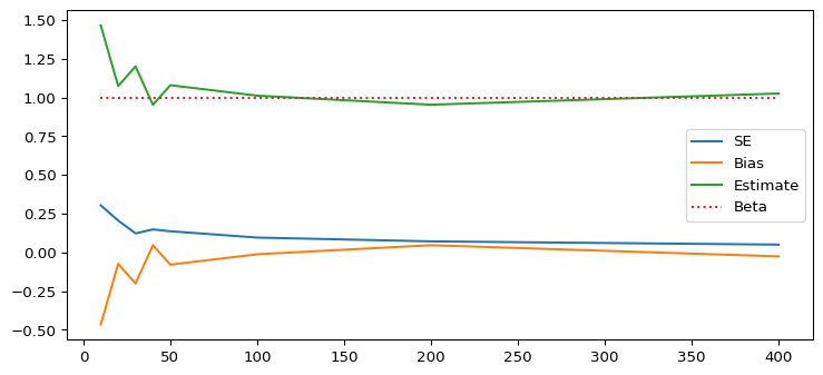
Solution to Exercise 3.3.
# Input: nobs, nrep
# Given a number of observation, we want to repeat the simulation R times
# Output: mean Bias, SE and Estimates

def SIM(n, R):

    beta = 1
    Estim = np.zeros(R)
    Bias = np.zeros(R)
    SE = np.zeros(R)


    for i in range(0,R):
        outcome, regressor = DGP(beta, n)
        ols = sm.OLS(outcome, regressor)
        ols = ols.fit()
        Estim[i] = ols.params[0]
        Bias[i] = beta - ols.params[0]
        SE[i] = ols.bse[0]

    mBias = np.mean(Bias)
    mSE = np.mean(SE)
    mEstim = np.mean(Estim)

return mBias, mSE, mEstimSIM(20, 10)(np.float64(-0.049914925213042714),
np.float64(0.21797594035041126),
np.float64(1.0499149252130426))# Results if we use a loop
R = 50
n = 100
beta = 1
Estim = np.zeros(R)
Bias = np.zeros(R)
SE = np.zeros(R)
np.random.seed(2)
for i in range(0,R):
outcome, regressor = DGP(beta, n)
ols = sm.OLS(outcome, regressor)
ols = ols.fit()
Estim[i] = ols.params[0]
Bias[i] = beta - ols.params[0]
SE[i] = ols.bse[0]
print(np.mean(Bias))
print(np.mean(SE))
print(np.mean(Estim))0.005504440656150831
0.09876240048185254
0.9944955593438491# With SIM Function
np.random.seed(2)
SIM(100, 50)(np.float64(0.005504440656150831),
np.float64(0.09876240048185254),
np.float64(0.9944955593438491))np.random.seed(1234)
R = 100
beta = 1
nobs = [10, 20, 30, 40, 50, 100, 200, 400]
# We need to declare objects to save the average results per nobs
AvgBias = np.zeros(len(nobs))
AvgSE = np.zeros(len(nobs))
AvgEstim = np.zeros(len(nobs))# First, let us simply extract the estimates in every repetition.
np.random.seed(1234)
for i in range(0,len(nobs)):
n = nobs[i]
AvgBias[i], AvgSE[i], AvgEstim[i] = SIM(n, R)fig = plt.figure(figsize=(9, 4))
plt.plot(nobs, AvgSE, label = "SE")
plt.plot(nobs, AvgBias, label = "Bias")
plt.plot(nobs, AvgEstim, label = "Estimates")
plt.title("Results, Averaged over 100 Repetitions")
plt.legend()
plt.show()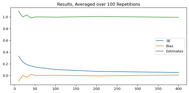
Solution to Exercise 3.4.
def SIM2(n, R):

    beta = 1
    Estim = np.zeros(R)

    for i in range(0,R):
        outcome, regressor = DGP(beta, n)
        ols = sm.OLS(outcome, regressor)
        ols = ols.fit()
        Estim[i] = ols.params[0]

    return Estim
R = 1000
res10 = SIM2(10, R)
res20 = SIM2(20, R)
res50 = SIM2(50, R)
res100 = SIM2(100, R)We repeat the simulation from above. But now, we need to save the \(\hat{\beta}\) so that we can compute \(\sqrt{n}(\hat{\beta}-\beta)\). We can illustrate the results by generating a bar plot similar to that in Lecture 1.
# Modify the SIM Function

def SIM2(n, R):

    beta = 1
    Estim = np.zeros(R)

    for i in range(0,R):
        outcome, regressor = DGP(beta, n)
        ols = sm.OLS(outcome, regressor)
        ols = ols.fit()
        Estim[i] = ols.params[0]

    return Estim
R = 1000
res10 = SIM2(10, R)
res20 = SIM2(20, R)
res50 = SIM2(50, R)
res100 = SIM2(100, R)We can already show that \(\hat{\beta}\) is \(\hat{\beta} \sim N(\beta,\sigma^2_{\hat{\beta}})\)
fig = plt.figure(figsize=(9, 4))
bins = np.linspace(-0, 2, 201)
plt.hist(res10, bins=bins,density=True,label='n = 10', color = "green")
plt.hist(res20, bins=bins,density=True,label='n = 20', color = "yellow")
plt.hist(res50, bins=bins,density=True,label='n = 50', color = "red")
plt.hist(res100, bins=bins,density=True,label='n = 100', color = "blue")
plt.legend()

plt.show()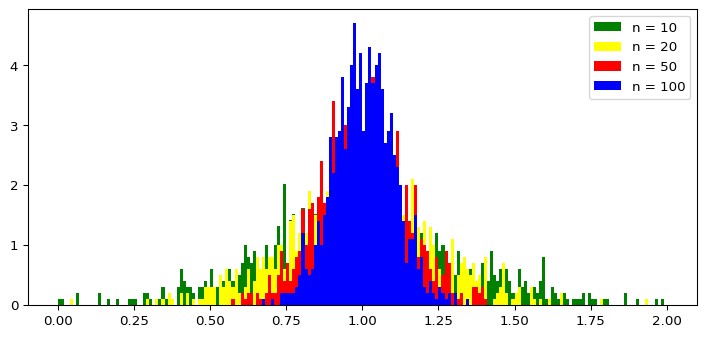
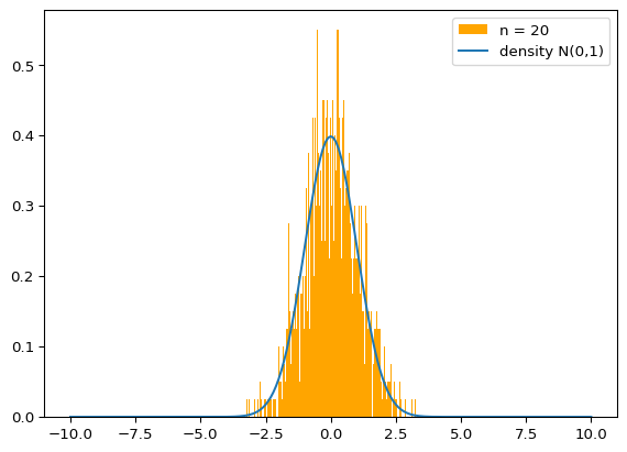
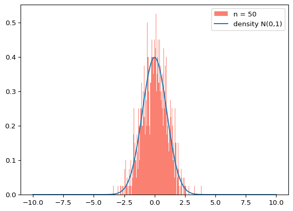
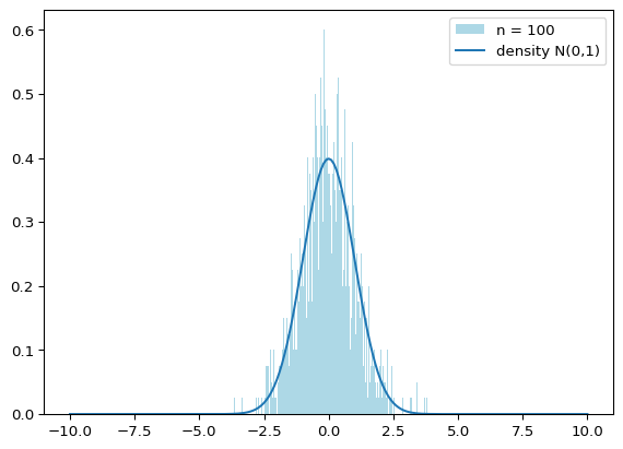
We want to illustrate that \(\sqrt{n}(\hat{\beta} - \beta) \xrightarrow[]{d} N(0,1)\).
res10 = np.sqrt(10)*( SIM2(10, R) - beta)
res20 = np.sqrt(20)*( SIM2(20, R) - beta)
res50 = np.sqrt(50)*( SIM2(50, R) - beta)
res100 = np.sqrt(100)*( SIM2(100, R) - beta)
from scipy.stats import norm
xy = np.linspace(-10, 10, 201)
y = norm.pdf(xy, 0, 1)fig = plt.figure(4)
bins = np.linspace(-4, 4, 201)
plt.hist(res10, bins=bins,density=True,label='n = 10', color = "lightgreen")
plt.plot(xy, y, '-', linewidth=1.5, label='density N(0,1)') # adding the density
plt.legend()
plt.show()
plt.hist(res20, bins=bins,density=True,label='n = 20', color = "orange")
plt.plot(xy, y, '-', linewidth=1.5, label='density N(0,1)') # adding the density
plt.legend()
plt.show()
plt.hist(res50, bins=bins,density=True,label='n = 50', color = "salmon")
plt.plot(xy, y, '-', linewidth=1.5, label='density N(0,1)') # adding the density
plt.legend()
plt.show()
plt.hist(res100, bins=bins,density=True,label='n = 100', color = "lightblue")
plt.plot(xy, y, '-', linewidth=1.5, label='density N(0,1)') # adding the density
plt.legend()
plt.show()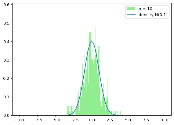
Solution to Exercise 3.5. (optional)
The type-1-error control says that, if the \(H_0\) is true, we reject the \(H_0\) with less than probability \(\alpha\).
Hence, we need to simulate a situation where the null hypothesis is true and count how many times we reject the \(H_0\). We should not reject more often than in \(\alpha\) percent of the cases.
In our example, we test \(H_0: \beta = 0\) vs. \(H_A: \beta \neq 0\).
The test is rejected if the p-value is smaller than \(\alpha\).
# Modify the SIM Function
# i) the H0 needs to be true (i.e. beta = 0)
# ii) we want to get the p-values at output

def SIM3(n, R):

    beta = 0
    Pvalues = np.zeros(R)

    for i in range(0,R):
        outcome, regressor = DGP(beta, n)
        ols = sm.OLS(outcome, regressor)
        ols = ols.fit()
        Pvalues[i] = ols.pvalues[0]

    return Pvalues
n = 100
R = 10000
pvals = SIM3(n,R)alpha = 0.05
level = np.sum(pvals<0.05)/R
print("Level of the t-test:", level)Level of the t-test: 0.0528