Statistical Programming: Problem Set 4

Exercise 1: Support Vector Machines

Explain in your own words how the Support Vector Machines work. You do not need to provide a mathematical description, an explanation of the basic theory is fine. Explain the usage of slack variables. Why do we need them?
Compare SVMs to Logistic Regression. How do they differ?

Exercise 2: Logistic Regression

Now load the first classification_1 dataset. The data consist of two features and a classification variable.

Solution:

import pandas as pd
import numpy as np
from sklearn.linear_model import LogisticRegression
import matplotlib.pyplot as plt

# Load data
data = pd.read_csv(r"https://raw.githubusercontent.com/JanTeichertKluge/data-statprog/refs/heads/main/data/classification_1.csv", sep=';', na_values=".")

# Part 1: Number of classes
num_classes = data['class'].nunique()  # Should be 2
print(f"Number of classes: {num_classes}")

# Part 2: Logistic Regression
X = pd.DataFrame(data, columns=['length', 'height']).values
y = pd.DataFrame(data, columns=['class']).values.flatten()

logistic_model = LogisticRegression(penalty='l2', solver='liblinear')
logistic_model.fit(X, y)

y_pred = logistic_model.predict(X)
error_rate = np.mean(y_pred != y)
print(f"Error rate: {error_rate:.4f}")

# Part 3: Visualization
plt.scatter(X[y==0, 0], X[y==0, 1], c='red', label='Class 0')
plt.scatter(X[y==1, 0], X[y==1, 1], c='blue', label='Class 1')
plt.xlabel('Length')
plt.ylabel('Height')
plt.legend()
plt.show()

# Part 4: The data appears to be circularly distributed
# Logistic regression (linear) may not work well
# Try SVM with RBF kernel for better results

Solution:

Logistic regression is a linear classifier. Hence the two classes can not be separated.

Exercise 3: Wine classification

Now load the wine dataset. The dataset contains information on the chemical composition of wines. You can load the data via

Make yourself familiar with the data. How many different wine types are contained in the sample? How many different features and observations are included?
Use the train_test_split function (test_size = 0.2, random_state=0) to split your your data into a training and a testing sample.
Try to classify your data with the \(k\)-nearest neighbor classification. Use different weights and number of neighbors to minimize your empirical error rate.
Try to improve on you result by using random forests.
Can you try to determine two of the most important features(determined by the attribute .feature_importances_ ) that can be used to seperate the results?

Solution:

import pandas as pd
import numpy as np
from sklearn.datasets import load_wine
from sklearn.model_selection import train_test_split
from sklearn import neighbors
from sklearn.ensemble import RandomForestClassifier

# Load data
dataset = load_wine()
df = pd.DataFrame(dataset.data, columns=dataset.feature_names)
df['Type'] = dataset.target

# Part 1: Explore
print("Number of wine types:", len(df['Type'].unique()))  # 3
print("Number of features:", len(dataset.feature_names))  # 13
print("Number of observations:", len(df))  # 178

# Part 2: Split
X_train, X_test, y_train, y_test = train_test_split(
    dataset.data, dataset.target, test_size=0.2, random_state=0
)

# Part 3: KNN
knn_uniform = neighbors.KNeighborsClassifier(n_neighbors=10, weights='uniform')
knn_uniform.fit(X_train, y_train)
knn_uniform_error = np.mean(knn_uniform.predict(X_test) != y_test)
print(f"KNN error rate: {knn_uniform_error:.4f}")

# Part 4: Random Forest
rf_model = RandomForestClassifier(max_depth=5, random_state=0)
rf_model.fit(X_train, y_train)
rf_error = np.mean(rf_model.predict(X_test) != y_test)
print(f"Random Forest error rate: {rf_error:.4f}")

# Part 5: Feature importance
importance_df = pd.DataFrame(
    [rf_model.feature_importances_],
    index=["importance"],
    columns=dataset.feature_names
)
print(importance_df.T.sort_values(by='importance', ascending=False))

Alternative Solutions:

Exercise 4: Digits classification

The (famous) MNIST dataset contains 70.000 observations of an image of a handwritten digit. Each observation consists \(784\) features (grey level) which correspond to a \(28\times28\) image. The MNIST data set is very popular to train and test algorithms in machine learning (see http://yann.lecun.com/exdb/mnist/ )

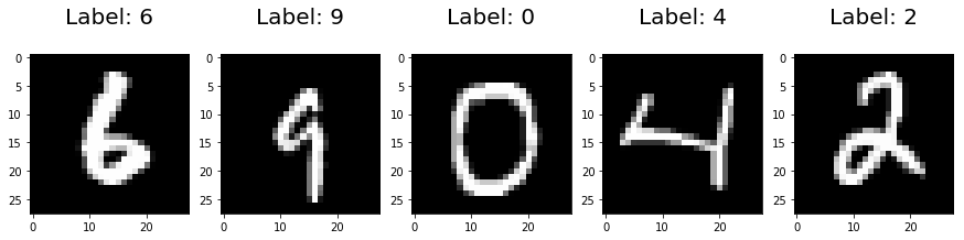
Due to time constraints we process the just a subset with a reduced number of features. At first load the digits datastet.

Again, make yourself familiar with the data. How many different features and observations are included?
Use the train_test_split function (test_size = 0.2, random_state=0) to split your your data into a training and a testing sample.
Try to classify your data with the support vector machines. Use different kernels and other tuning parameters minimize your empirical error rate.

Solution:

import pandas as pd
import numpy as np
from sklearn.datasets import load_digits
from sklearn.model_selection import train_test_split
from sklearn import svm

# Load data
dataset = load_digits()
df = pd.DataFrame(dataset.data)
df['Digit'] = dataset.target

# Part 1: Explore
print("Number of features:", df.shape[1] - 1)  # 64
print("Number of observations:", df.shape[0])  # 1797

# Part 2: Split
X_train, X_test, y_train, y_test = train_test_split(
    dataset.data, dataset.target, test_size=0.2, random_state=0
)

# Part 3: SVM with different kernels
# Linear kernel
svm_linear = svm.SVC(kernel='linear', C=2)
svm_linear.fit(X_train, y_train)
linear_error = np.mean(svm_linear.predict(X_test) != y_test)
print(f"Linear kernel error rate: {linear_error:.4f}")

# Polynomial kernel
svm_poly = svm.SVC(kernel='poly', degree=2, C=2, gamma='auto')
svm_poly.fit(X_train, y_train)
poly_error = np.mean(svm_poly.predict(X_test) != y_test)
print(f"Polynomial kernel error rate: {poly_error:.4f}")

# RBF kernel
svm_rbf = svm.SVC(kernel='rbf', C=2, gamma='auto')
svm_rbf.fit(X_train, y_train)
rbf_error = np.mean(svm_rbf.predict(X_test) != y_test)
print(f"RBF kernel error rate: {rbf_error:.4f}")