Statistical Programming: Problem Set 4

Author

Affiliation

Philipp Bach, Jan Teichert-Kluge

University of Hamburg

Exercise 1: Support Vector Machines

Explain in your own words how the Support Vector Machines work. You do not need to provide a mathematical description, an explanation of the basic theory is fine. Explain the usage of slack variables. Why do we need them?
Compare SVMs to Logistic Regression. How do they differ?

Solution

Explain in your own words

Support Vector Machines (SVMs) are a class of supervised learning algorithms used for classification and regression tasks. They work by finding the optimal hyperplane that separates different classes in the feature space. The key idea is to maximize the margin between the nearest data points of the different classes, known as support vectors.

In a nutshell, SVMs aim to find the best possible line (or hyperplane in higher dimensions) that divides data points into classes. This line should be positioned in such a way that it maximizes the distance between the nearest data points of each class, thus creating a wide margin. This wide margin helps in generalizing the classification to new, unseen data points.

For datasets that are linearly separable, SVMs identify the hyperplane that perfectly separates the classes. However, in real-world scenarios where data may not be perfectly separable, SVMs introduce the concept of slack variables, which allow for some misclassification. This is known as the soft-margin approach, where the algorithm seeks to find a balance between maximizing the margin and minimizing misclassification errors.

One of the remarkable features of SVMs is the kernel trick, which allows them to handle non-linear relationships between features. By implicitly mapping the input data into a higher-dimensional feature space, SVMs can effectively find linear separation boundaries in this transformed space. This is achieved through kernel functions, which compute the inner product between transformed feature vectors. Popular kernel functions include polynomial kernels and radial basis function kernels.

In summary, SVMs offer a powerful framework for classification tasks by finding the optimal hyperplane that separates different classes, with the flexibility to handle both linear and non-linear relationships between features.

Compare the SVM to the Logistic Regression

Logistic regression was discussed in the lecture. Compare the SVM just presented with the logistic regression and give at least 2 differences between them.

Solution

Logistic Regression

Logistic Regression, also known as logit models, is another popular classification algorithm. Unlike SVMs, which aim to find the maximum margin hyperplane, Logistic Regression models the probability of belonging to a particular class using a logistic function.

Differences

Decision Boundary: SVMs aim to find the hyperplane with the maximum margin, while Logistic Regression models the probability directly, resulting in a linear decision boundary.
Nonlinearity: SVMs can handle nonlinear relationships through the kernel trick, whereas Logistic Regression assumes a linear relationship between features and the log-odds of the target variable.
Interpretability: Logistic regression provides probabilities for each class, making it more interpretable in terms of likelihoods, while SVM provides a clear separation boundary.

Exercise 2: Logistic Regression

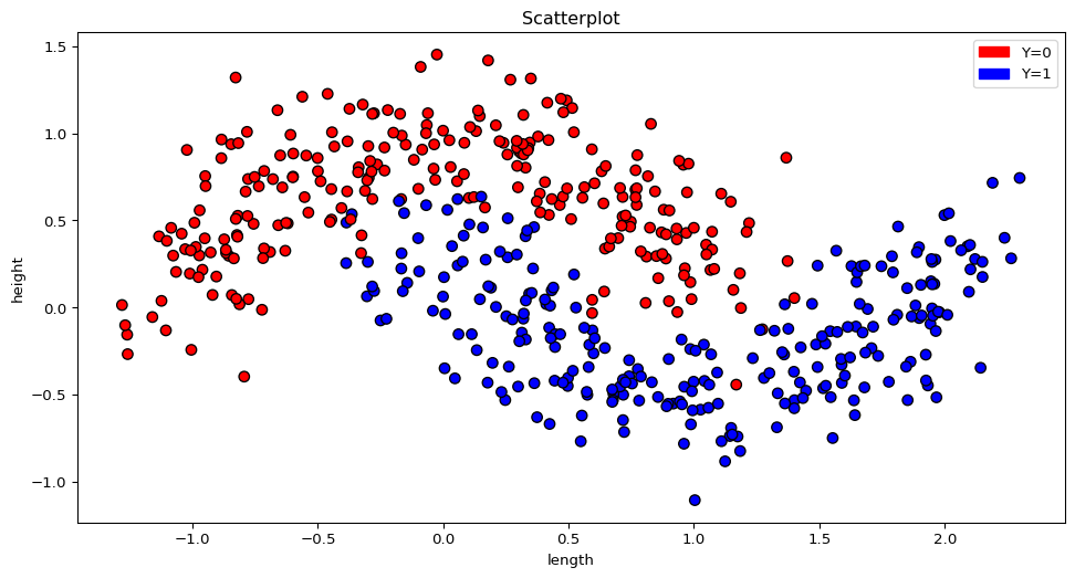
Now load the first classification_1 dataset. The data consist of two features and a classification variable.

How many different classes are contained in the dataset? (Hint: help(pd.unique))
Use logistic regression to separate both classes and measure the error rate on the training set.
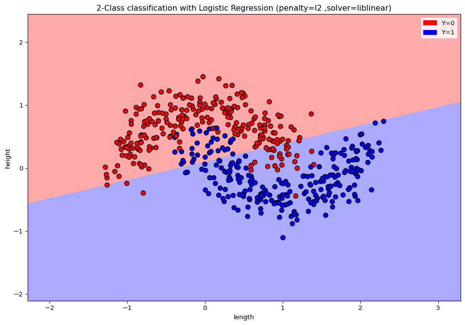
Try to visualize the data with matplotlib. Can you explain the results from the logistic regression?
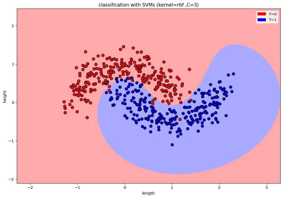
Which method could be better suited for this task? Try to improve on the error rate.

Solution:

import pandas as pd
import numpy as np
data = pd.read_csv('https://raw.githubusercontent.com/JanTeichertKluge/data-statprog/refs/heads/main/data/classification_1.csv', sep=';', na_values=".")
data.head()

	length	height	class
0	0.302402	0.896238	0.0
1	-0.385983	0.487310	1.0
2	0.190209	0.113254	1.0
3	1.714572	-0.110330	1.0
4	1.967063	-0.515801	1.0

data.shape

(500, 3)

data['class'].unique()

array([0., 1.])

#help(set)
set(pd.DataFrame(data, columns=['class']).values.flatten())

{np.float64(0.0), np.float64(1.0)}

from sklearn.linear_model import LogisticRegression
X = pd.DataFrame(data, columns=['length','height'])
X = X.values
y = pd.DataFrame(data, columns=['class'])
y = y.values
y = y.flatten()
logisticRegr = LogisticRegression(penalty = 'l2', solver = 'liblinear')
model = logisticRegr.fit(X, y)
y_score = model.predict(X)
#Score function from scikit:
print('Error rate:', np.mean(np.not_equal(model.predict(X),y)))

Error rate: 0.134

/home/runner/work/Statistical-Programming/Statistical-Programming/.venv/lib/python3.11/site-packages/sklearn/linear_model/_logistic.py:1135: FutureWarning:

'penalty' was deprecated in version 1.8 and will be removed in 1.10. To avoid this warning, leave 'penalty' set to its default value and use 'l1_ratio' or 'C' instead. Use l1_ratio=0 instead of penalty='l2', l1_ratio=1 instead of penalty='l1', and C=np.inf instead of penalty=None.

# Alternatively
print(np.mean(np.array(model.predict(X) != y)))

0.134

import matplotlib.pyplot as plt
from matplotlib.colors import ListedColormap
import matplotlib.patches as mpatches

plot_symbol_size = 50
cmap_bold  = ListedColormap(['#FF0000', '#0000FF'])
plt.figure(figsize=(12,6))
plt.scatter(X[:, 0], X[:, 1], s=plot_symbol_size, c=y, cmap=cmap_bold, edgecolor = 'black')
plt.xlabel("length")
plt.ylabel("height")
plt.title("Scatterplot")
patch0 = mpatches.Patch(color='#FF0000', label='Y=0')
patch1 = mpatches.Patch(color='#0000FF', label='Y=1')
plt.legend(handles=[patch0, patch1])
plt.show()

import matplotlib.cm as cm
from matplotlib.colors import ListedColormap, BoundaryNorm
import matplotlib.patches as mpatches
Y = y
pen = 'l2'
solv = 'liblinear'
# Create color maps
cmap_light = ListedColormap(['#FFAAAA', '#AAAAFF'])
cmap_bold  = ListedColormap(['#FF0000', '#0000FF'])

# Plot the decision boundary by assigning a color in the color map to each mesh point.
mesh_step_size = .01  # step size in the mesh
plot_symbol_size = 50
    
x_min, x_max = X[:, 0].min() - 1, X[:, 0].max() + 1
y_min, y_max = X[:, 1].min() - 1, X[:, 1].max() + 1
xx, yy = np.meshgrid(np.arange(x_min, x_max, mesh_step_size),
                         np.arange(y_min, y_max, mesh_step_size))
Z = model.predict(np.c_[xx.ravel(), yy.ravel()])

# Put the result into a color plot
Z = Z.reshape(xx.shape)
plt.figure(3,figsize=(12,8))
plt.pcolormesh(xx, yy, Z, cmap=cmap_light)

# Plot training points
plt.scatter(X[:, 0], X[:, 1], s=plot_symbol_size, c=Y, cmap=cmap_bold, edgecolor = 'black')
plt.xlim(xx.min(), xx.max())
plt.ylim(yy.min(), yy.max())

patch0 = mpatches.Patch(color='#FF0000', label='Y=0')
patch1 = mpatches.Patch(color='#0000FF', label='Y=1')
plt.legend(handles=[patch0, patch1])

plt.xlabel('length')
plt.ylabel('height')
plt.title("2-Class classification with Logistic Regression (penalty=%s ,solver=%s)" % (pen, solv))    
plt.show()

/home/runner/work/Statistical-Programming/Statistical-Programming/.venv/lib/python3.11/site-packages/IPython/core/pylabtools.py:170: UserWarning:

Creating legend with loc="best" can be slow with large amounts of data.

Logistic regression is a linear classifier. Hence the two classes can not be separated. (obige Grafik als Veranschaulichung)

from sklearn import svm
supvecma = svm.SVC(kernel = 'rbf', C = 3)
model = supvecma.fit(X, Y)
print('Error rate:', np.mean(np.not_equal(model.predict(X),y)))

Error rate: 0.03

import matplotlib.cm as cm
from matplotlib.colors import ListedColormap, BoundaryNorm
import matplotlib.patches as mpatches
Y = y
# Create color maps
cmap_light = ListedColormap(['#FFAAAA', '#AAAAFF'])
cmap_bold  = ListedColormap(['#FF0000', '#0000FF'])

# Plot the decision boundary by assigning a color in the color map to each mesh point.
mesh_step_size = .01  # step size in the mesh
plot_symbol_size = 50
    
x_min, x_max = X[:, 0].min() - 1, X[:, 0].max() + 1
y_min, y_max = X[:, 1].min() - 1, X[:, 1].max() + 1
xx, yy = np.meshgrid(np.arange(x_min, x_max, mesh_step_size),
                         np.arange(y_min, y_max, mesh_step_size))
Z = model.predict(np.c_[xx.ravel(), yy.ravel()])

# Put the result into a color plot
Z = Z.reshape(xx.shape)
plt.figure(3,figsize=(12,8))
plt.pcolormesh(xx, yy, Z, cmap=cmap_light)

# Plot training points
plt.scatter(X[:, 0], X[:, 1], s=plot_symbol_size, c=Y, cmap=cmap_bold, edgecolor = 'black')
plt.xlim(xx.min(), xx.max())
plt.ylim(yy.min(), yy.max())

patch0 = mpatches.Patch(color='#FF0000', label='Y=0')
patch1 = mpatches.Patch(color='#0000FF', label='Y=1')
plt.legend(handles=[patch0, patch1])

plt.xlabel('length')
plt.ylabel('height')
plt.title("classification with SVMs (kernel=rbf ,C=3)" )    
plt.show()

Exercise 3: Wine classification

Now load the wine dataset. The dataset contains information on the chemical composition of wines. You can load the data via

from sklearn.datasets import load_wine
dataset = load_wine()

Make yourself familiar with the data. How many different wine types are contained in the sample? How many different features and observations are included?
Use the train_test_split function (test_size = 0.2, random_state=0) to split your your data into a training and a testing sample.
Try to classify your data with the \(k\)-nearest neighbor classification. Use different weights and number of neighbors to minimize your empirical error rate.
Try to improve on you result by using random forests.
Can you try to determine two of the most important features(determined by the attribute .feature_importances_ ) that can be used to seperate the results?

Solution

import pandas as pd
import numpy as np
from sklearn.datasets import load_wine
dataset = load_wine()
df = pd.DataFrame(dataset.data, columns=dataset.feature_names)
df['Type'] = dataset.target
df.head()

	alcohol	malic_acid	ash	alcalinity_of_ash	magnesium	total_phenols	flavanoids	nonflavanoid_phenols	proanthocyanins	color_intensity	hue	od280/od315_of_diluted_wines	proline
0	14.23	1.71	2.43	15.6	127.0	2.80	3.06	0.28	2.29	5.64	1.04	3.92	1065.0
1	13.20	1.78	2.14	11.2	100.0	2.65	2.76	0.26	1.28	4.38	1.05	3.40	1050.0
2	13.16	2.36	2.67	18.6	101.0	2.80	3.24	0.30	2.81	5.68	1.03	3.17	1185.0
3	14.37	1.95	2.50	16.8	113.0	3.85	3.49	0.24	2.18	7.80	0.86	3.45	1480.0
4	13.24	2.59	2.87	21.0	118.0	2.80	2.69	0.39	1.82	4.32	1.04	2.93	735.0

print(np.shape(df))
print(dataset.target)
#set(pd.DataFrame(df, columns=['Type']).values.flatten())
print(df['Type'].unique())

(178, 14)
[0 0 0 0 0 0 0 0 0 0 0 0 0 0 0 0 0 0 0 0 0 0 0 0 0 0 0 0 0 0 0 0 0 0 0 0 0
 0 0 0 0 0 0 0 0 0 0 0 0 0 0 0 0 0 0 0 0 0 0 1 1 1 1 1 1 1 1 1 1 1 1 1 1 1
 1 1 1 1 1 1 1 1 1 1 1 1 1 1 1 1 1 1 1 1 1 1 1 1 1 1 1 1 1 1 1 1 1 1 1 1 1
 1 1 1 1 1 1 1 1 1 1 1 1 1 1 1 1 1 1 1 2 2 2 2 2 2 2 2 2 2 2 2 2 2 2 2 2 2
 2 2 2 2 2 2 2 2 2 2 2 2 2 2 2 2 2 2 2 2 2 2 2 2 2 2 2 2 2 2]
[0 1 2]

from sklearn.model_selection import train_test_split
X_train, X_test, y_train, y_test = train_test_split(dataset.data, dataset.target, test_size=0.2, random_state=0)

from sklearn import neighbors
neighb = neighbors.KNeighborsClassifier(n_neighbors = 10, weights = 'uniform')
model = neighb.fit(X_train, y_train)
print('Error rate:', np.mean(np.not_equal(model.predict(X_test),y_test)))

Error rate: 0.2777777777777778

from sklearn import neighbors
neighb = neighbors.KNeighborsClassifier(n_neighbors = 10, weights = 'distance')
model = neighb.fit(X_train, y_train)
print('Error rate:', np.mean(np.not_equal(model.predict(X_test),y_test)))

Error rate: 0.25

import pandas as pd
from sklearn.ensemble import RandomForestClassifier
randforest = RandomForestClassifier(max_depth=5, random_state=0)
model = randforest.fit(X_train, y_train)
print('Error rate:', np.mean(np.not_equal(model.predict(X_test),y_test)))
importance=pd.DataFrame([model.feature_importances_],index=["importance"], columns=dataset.feature_names)
importance

Error rate: 0.027777777777777776

	alcohol	malic_acid	ash	alcalinity_of_ash	magnesium	total_phenols	flavanoids	nonflavanoid_phenols	proanthocyanins	color_intensity	hue	od280/od315_of_diluted_wines	proline
importance	0.103923	0.031157	0.012805	0.020604	0.019559	0.059636	0.156013	0.019817	0.036109	0.174127	0.066472	0.14339	0.156389

Exercise 4: Digits classification

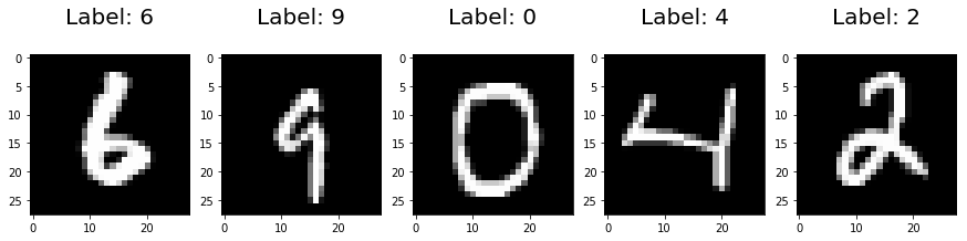
The (famous) MNIST dataset contains 70.000 observations of an image of a handwritten digit. Each observation consists \(784\) features (grey level) which correspond to a \(28\times28\) image. The MNIST data set is very popular to train and test algorithms in machine learning (see http://yann.lecun.com/exdb/mnist/ )

Due to time constraints we process the just a subset with a reduced number of features. At first load the digits datastet.

import pandas as pd
from sklearn.datasets import load_digits
dataset = load_digits()
df = pd.DataFrame(dataset.data)
df['Digit'] = dataset.target
df[0:3]

	2	3	4	5	...	58	59	60	61	62	Digit
0	5.0	13.0	9.0	1.0	...	6.0	13.0	10.0	0.0	0.0	0
1	0.0	12.0	13.0	5.0	...	0.0	11.0	16.0	10.0	0.0	1
2	0.0	4.0	15.0	12.0	...	0.0	3.0	11.0	16.0	9.0	2

3 rows × 65 columns

Again, make yourself familiar with the data. How many different features and observations are included?
Use the train_test_split function (test_size = 0.2, random_state=0) to split your your data into a training and a testing sample.
Try to classify your data with the support vector machines. Use different kernels and other tuning parameters minimize your empirical error rate.

Solution:

import numpy as np
np.shape(df)

(1797, 65)

from sklearn.model_selection import train_test_split
X_train, X_test, y_train, y_test = train_test_split(dataset.data,dataset.target, test_size=0.2, random_state=0)

from sklearn import svm
supvecma = svm.SVC(kernel = 'linear', C = 2)
model = supvecma.fit(X_train, y_train)
print('Error rate:', np.mean(np.not_equal(model.predict(X_test),y_test)))

Error rate: 0.022222222222222223

from sklearn import svm
supvecma = svm.SVC(kernel = 'poly',degree =2, C = 2, gamma = 'auto')
model = supvecma.fit(X_train, y_train)
print('Error rate:', np.mean(np.not_equal(model.predict(X_test),y_test)))

Error rate: 0.011111111111111112